GOM23_OilHeatWave_Analysis

Author

Meagan Sonsel

Published

November 4, 2025

library(tidyverse);library(phyloseq);

── Attaching core tidyverse packages ──────────────────────── tidyverse 2.0.0 ──
✔ dplyr     1.1.4     ✔ readr     2.1.5
✔ forcats   1.0.0     ✔ stringr   1.5.2
✔ ggplot2   4.0.0     ✔ tibble    3.3.0
✔ lubridate 1.9.4     ✔ tidyr     1.3.1
✔ purrr     1.1.0     
── Conflicts ────────────────────────────────────────── tidyverse_conflicts() ──
✖ dplyr::filter() masks stats::filter()
✖ dplyr::lag()    masks stats::lag()
ℹ Use the conflicted package (<http://conflicted.r-lib.org/>) to force all conflicts to become errors

library(compositions); library(patchwork)

Welcome to compositions, a package for compositional data analysis.
Find an intro with "? compositions"


Attaching package: 'compositions'

The following objects are masked from 'package:stats':

    anova, cor, cov, dist, var

The following object is masked from 'package:graphics':

    segments

The following objects are masked from 'package:base':

    %*%, norm, scale, scale.default

load(file = "input-data/asv_wtax_qc_GoM23_062025.RData", verbose = TRUE)

Loading objects:
  samples_too_low
  env_info
  asv_wide_cleaned
  asv_long_cleaned

env_info <- read.csv("input-data/metadata-gom-23.csv")

library(geosphere)
outflow_lat <- 28.95
outflow_long <- 89.39
outflow <- c(outflow_long, outflow_lat)

stn_info <- read.csv("input-data/manual_stn_classification.csv")

offshore_on_shore_order <- c(1, 2, 3, 4, 5, 9, 8, 7, 6, 10, 11, 12, 13, 14, 15)

transect_labels <- c("transect1", "transect1", "transect1", "transect1", "transect1", "transect2", "transect2", "transect2", "transect2", "transect3", "transect3", "transect3", "transect3", "transect3", "transect3")

depth_order <- as.character(sort((unique(env_info$DEPTH))))
depth_order_round <- as.character(sort(round(unique(env_info$DEPTH), digits = 0)))

env_info_mod <- env_info %>% 
  left_join(stn_info) %>% 
  mutate(STN_ORDER = factor(Station, levels = offshore_on_shore_order),
         TRANSECT = factor(Station, levels = offshore_on_shore_order, transect_labels),
         DEPTH_ORDER = factor(DEPTH, levels = rev(depth_order), labels = rev(depth_order_round))) %>% 
  mutate(DIST_OUTFLOW = distHaversine(cbind(Longitude, Latitude), cbind(outflow_long, outflow_lat)))

Joining with `by = join_by(Station)`

buffer_counts <- read.csv("input-data/OilRig_BufferCount - Sheet1.csv")

env_info_oil <- env_info_mod %>%
  left_join(buffer_counts, by = "Station")

asv_long_clean_wtax <- asv_long_cleaned %>% 
  filter(Domain == "Eukaryota") %>% 
  filter(Supergroup != "nucl") %>% 
  mutate(DIVISION = case_when(
    Subdivision == "X" ~ "Unannotated",
    is.na(Subdivision) ~ "Unannotated",
    TRUE ~ Subdivision
  )) %>% 
  # Goal is to combine Subdivision-Class
  mutate(SUPERGROUP_CLASS = case_when(
    ## High level NAs at the supergroup and division level
    (is.na(Division) & !is.na(Supergroup)) ~ paste(Supergroup, "Unannotated", sep = "-"),
    (is.na(Division) & is.na(Supergroup)) ~ "Eukaryote-Unannotated",
    (is.na(Subdivision)) ~ paste(Supergroup, "Unannotated", sep = "-"),
    (is.na(Class) & !is.na(Subdivision)) ~ paste(Subdivision, "Unannotated", sep = "-"),
    #
    (Subdivision == "X") ~ paste(Division, "Unannotated", sep = "-"),
    (Class == "X") ~ paste(Subdivision, "Unannotated", sep = "-"),
    TRUE ~ paste(Subdivision, Class, sep = "-"))) %>% 
  mutate(Supergroup_simplified = case_when(
    Supergroup == "TSAR" ~ paste("TSAR", Subdivision, sep = "-"),
    Supergroup == "Obazoa" ~ paste("Obazoa", DIVISION, sep = "-"),
    TRUE ~ Supergroup
  )) %>% 
  left_join(env_info_oil)

Joining with `by = join_by(SAMPLES)`

asv_long_avg_wtax <- asv_long_clean_wtax %>% 
  mutate(OilRig_Count = as.numeric(OilRig_Count),
         OilRig_Group = case_when(
           OilRig_Count >= 5 ~ "High",
           OilRig_Count >= 1 & OilRig_Count < 5 ~ "Medium",
           is.na(OilRig_Count) ~ "Unknown",
           OilRig_Count == 0 ~ "Low",
           TRUE ~ "Low"
         )) %>%
  mutate(OilRig_Group = factor(OilRig_Group, levels = c("Low","Medium","High","Unknown"))) %>%
  group_by(TRANSECT, PROX_TOSHORE, STN_ORDER, STN_CATEGORY_3, STN_CATEGORY_4, DEPTH_ORDER, FeatureID, stn, nisk, Station, Niskin, DEPTH, TEMP, SALINITY, OXYGEN, NH4, NO2, NO3, PO4, SIL, OilRig_Count, OilRig_Group, Taxon, DIVISION, SUPERGROUP_CLASS, Supergroup_simplified, Supergroup, Division, Subdivision, Class, Order, Family, Genus) %>% 
  summarise(MEAN_REPS_seq = mean(SEQUENCE_COUNT)) %>% 
  ungroup() %>% 
  unite(SAMPLE_ID, stn, nisk, sep = " ", remove = FALSE)

`summarise()` has grouped output by 'TRANSECT', 'PROX_TOSHORE', 'STN_ORDER',
'STN_CATEGORY_3', 'STN_CATEGORY_4', 'DEPTH_ORDER', 'FeatureID', 'stn', 'nisk',
'Station', 'Niskin', 'DEPTH', 'TEMP', 'SALINITY', 'OXYGEN', 'NH4', 'NO2',
'NO3', 'PO4', 'SIL', 'OilRig_Count', 'OilRig_Group', 'Taxon', 'DIVISION',
'SUPERGROUP_CLASS', 'Supergroup_simplified', 'Supergroup', 'Division',
'Subdivision', 'Class', 'Order', 'Family'. You can override using the `.groups`
argument.

# output_folder <- "C:\\Users\\msons\\OneDrive\\Documents\\GOM_23_ASV"
# file_name <- "asv_long_avg_wtax.csv"
# full_path <- file.path(output_folder, file_name)

# write.csv(asv_long_avg_wtax, full_path, row.names = FALSE)

# view(asv_long_avg_wtax)

Coastal Stations Supergroup Level

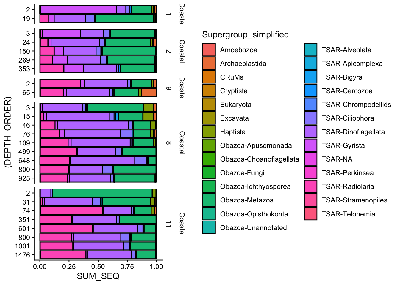
asv_long_avg_wtax %>%
  group_by(PROX_TOSHORE, TRANSECT, STN_ORDER, STN_CATEGORY_3, DEPTH_ORDER, SAMPLE_ID, DEPTH, TEMP, Supergroup_simplified) %>%
  summarise(SUM_SEQ = sum(MEAN_REPS_seq),
            ASV_COUNT = n()) %>%
  filter(STN_CATEGORY_3 == "Coastal") %>%
  ggplot(aes(y = (DEPTH_ORDER), x = SUM_SEQ, fill = Supergroup_simplified)) +
    geom_bar(stat = "identity", position = "fill", color = "black") +
  facet_grid(rows = vars(STN_CATEGORY_3, STN_ORDER), space = "free", scales = "free") +
  theme_classic() +theme(
    strip.background = element_blank(),
    axis.text = element_text(color = "black")
  )

`summarise()` has grouped output by 'PROX_TOSHORE', 'TRANSECT', 'STN_ORDER',
'STN_CATEGORY_3', 'DEPTH_ORDER', 'SAMPLE_ID', 'DEPTH', 'TEMP'. You can override
using the `.groups` argument.

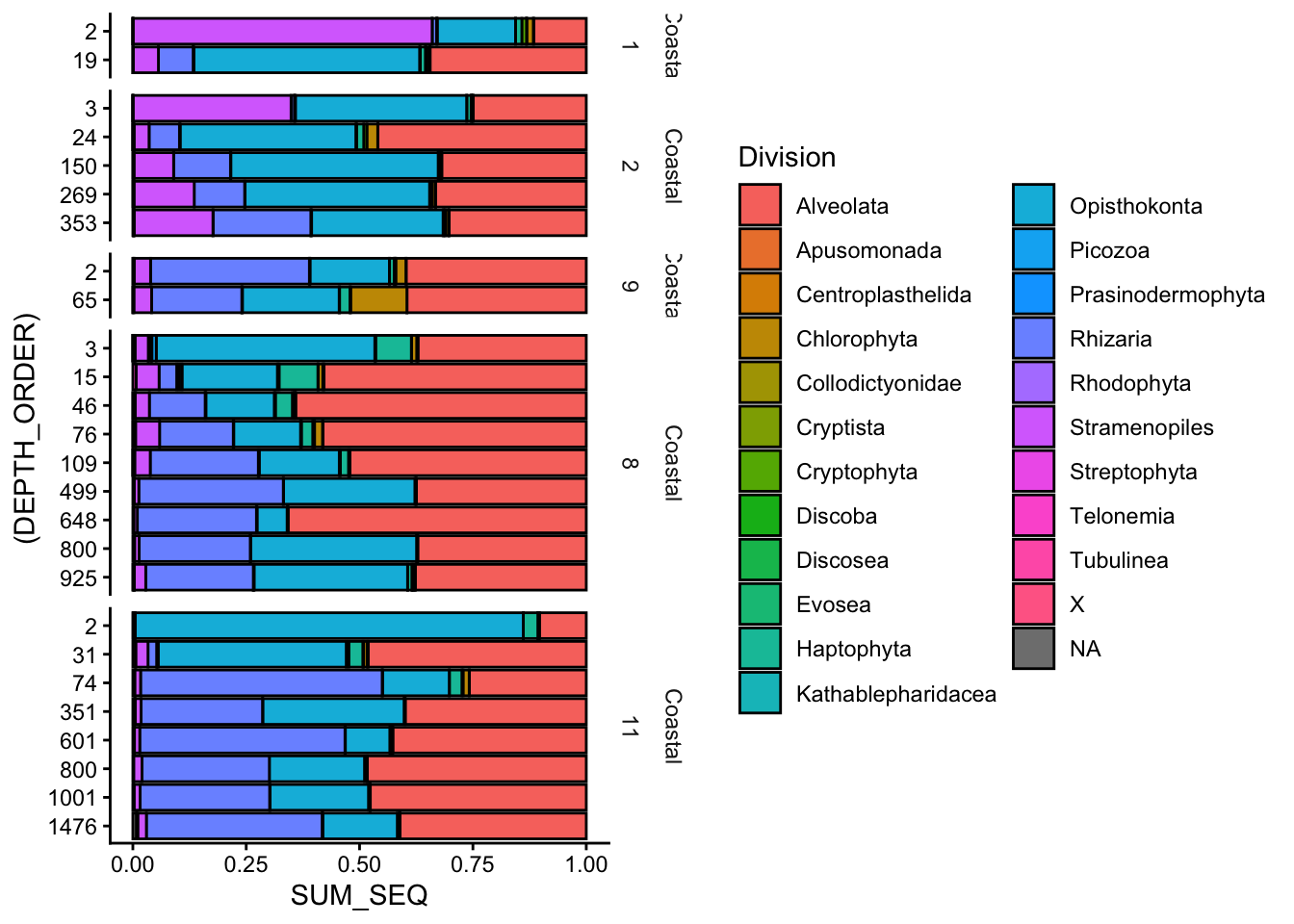
Coastal Stations Division Level

asv_long_avg_wtax %>%
  group_by(PROX_TOSHORE, TRANSECT, STN_ORDER, STN_CATEGORY_3, DEPTH_ORDER, SAMPLE_ID, DEPTH, TEMP, Division) %>%
  summarise(SUM_SEQ = sum(MEAN_REPS_seq),
            ASV_COUNT = n()) %>%
  filter(STN_CATEGORY_3 == "Coastal") %>%
  ggplot(aes(y = (DEPTH_ORDER), x = SUM_SEQ, fill = Division)) +
    geom_bar(stat = "identity", position = "fill", color = "black") +
  facet_grid(rows = vars(STN_CATEGORY_3, STN_ORDER), space = "free", scales = "free") +
  theme_classic() +theme(
    strip.background = element_blank(),
    axis.text = element_text(color = "black")
  )

`summarise()` has grouped output by 'PROX_TOSHORE', 'TRANSECT', 'STN_ORDER',
'STN_CATEGORY_3', 'DEPTH_ORDER', 'SAMPLE_ID', 'DEPTH', 'TEMP'. You can override
using the `.groups` argument.

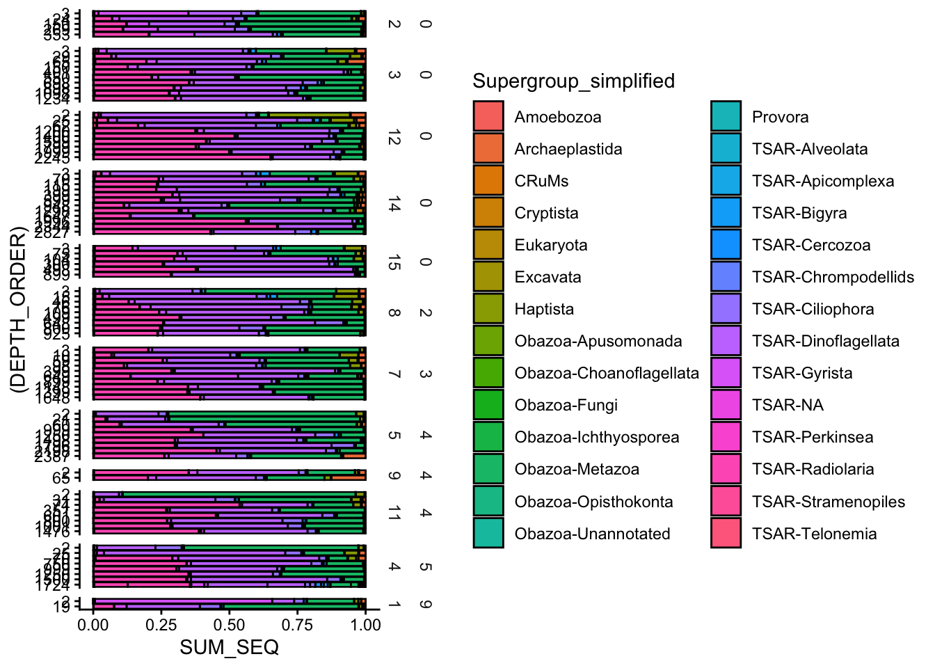
asv_long_avg_wtax %>%
  group_by(PROX_TOSHORE, TRANSECT, STN_ORDER, STN_CATEGORY_3, DEPTH_ORDER, SAMPLE_ID, DEPTH, TEMP, Supergroup_simplified, OilRig_Count) %>%
  summarise(SUM_SEQ = sum(MEAN_REPS_seq),
            ASV_COUNT = n()) %>%
  ggplot(aes(y = (DEPTH_ORDER), x = SUM_SEQ, fill = Supergroup_simplified)) +
    geom_bar(stat = "identity", position = "fill", color = "black") +
  facet_grid(rows = vars(OilRig_Count, STN_ORDER), space = "free", scales = "free") +
  theme_classic() +theme(strip.background = element_blank(), axis.text = element_text(color = "black"))

`summarise()` has grouped output by 'PROX_TOSHORE', 'TRANSECT', 'STN_ORDER',
'STN_CATEGORY_3', 'DEPTH_ORDER', 'SAMPLE_ID', 'DEPTH', 'TEMP',
'Supergroup_simplified'. You can override using the `.groups` argument.

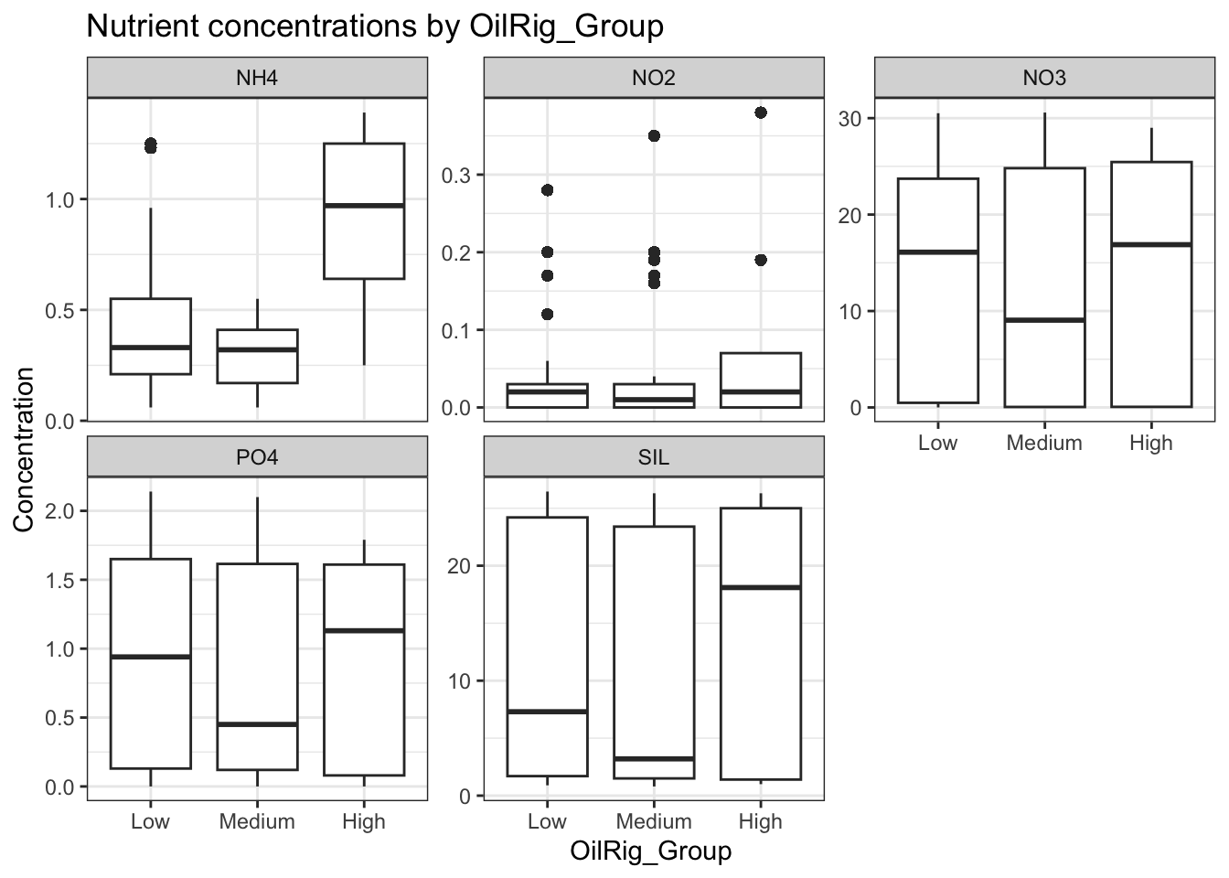
Nutrient Boxplots Arranged by Oil Rigs in 10 km Buffer Zone

asv_long_avg_wtax %>%
  rownames_to_column("Sample") %>%
  pivot_longer(cols = any_of(c("NO2","NO3","NH4","PO4","SIL")), names_to = "Nutrient", values_to = "Concentration") %>%
  ggplot(aes(x = OilRig_Group, y = Concentration)) +
  geom_boxplot() +
  facet_wrap(~ Nutrient, scales = "free_y") +
  theme_bw() +
  labs(title = "Nutrient concentrations by OilRig_Group")

asv_long_avg_wtax %>%
  rownames_to_column("Sample") %>%
  pivot_longer(cols = any_of(c("NO2","NO3","NH4","PO4","SIL")), names_to = "Nutrient", values_to = "Concentration") %>%
  ggplot(aes(x = STN_CATEGORY_3, y = Concentration)) +
  geom_boxplot() +
  facet_wrap(~ Nutrient, scales = "free_y") +
  theme_bw() +
  labs(title = "Nutrient concentrations by Station Category")

# install.packages("ggtern")
# library(ggtern)

# asv_long_avg_wtax %>%
#   mutate(Total = NH4 + PO4 +SIL,
#          NH4_per = (NH4/Total),
#          PO4_per = (PO4/Total),
#          SIL_per = (SIL/Total)) %>%
#   ggtern(aes(x = NH4_per, y = PO4_per, z = SIL_per, color = STN_CATEGORY_3)) +
#   geom_point()
# 
# asv_long_avg_wtax %>%
#   mutate(Total = NH4 + PO4 +SIL,
#          NH4_per = (NH4/Total),
#          PO4_per = (PO4/Total),
#          SIL_per = (SIL/Total)) %>%
#   ggtern(aes(x = NH4_per, y = PO4_per, z = SIL_per, color = OilRig_Group)) +
#   geom_point()