Protistan grazing analysis

1 Import & format data

Code below details how to import cell count (FLP count) information from Mid-Cayman Rise protistan grazing incubations, calculate cell abundances, estimate grazing rate, and cell biomass. This accompanies paper in review: Hu, S. K., Anderson, R. E., Pachiadaki, M. G., Edgcomb, V. P., Serres, M. H., Sylva, S. P., German, C. R., Seewald, J. S., Lang, S. Q., & Huber, J. A. (2023). Microbial eukaryotic predation pressure and biomass at deep-sea hydrothermal vents: Implications for deep-sea carbon cycling. In bioRxiv (p. 2023.08.11.552852). https://doi.org/10.1101/2023.08.11.552852

1.1 Set up working R environment

Load relevant libraries. A few libraries are loaded below in the code, but these are essential.

Code

library(tidyverse); library(cowplot); library(broom)
library(patchwork)

Set color schematic for the entire dataset. This is set so that all figures will be uniform for publication.

Code

vent_ids <- c("BSW","Plume", "LotsOShrimp", "Shrimpocalypse", 
              "ShrimpHole", "X18", "Rav2", "MustardStand", "OMT")
vent_fullname <- c("Background","Plume", "Lots 'O Shrimp", "Shrimpocalypse",  
                   "Shrimp Hole", "X-18", "Ravelin #2", "Mustard Stand", "Old Man Tree")
site_ids <- c("VD", "Piccard")
site_fullname <- c("Von Damm", "Piccard")
site_color <- c("#264653", "#E76F51")
names(site_color) <- site_fullname
whole_pal <- c("#264653", "#2A9D8F", "#E9C46A","#F4A261", "#E76F51")
extra <- c("#eae2b7", "#5f0f40", "#90be6d", "#941b0c", "#577590")

1.2 Import raw count data

Import eukaryotic cell count data from grazing experiments. In this section, we will calculate cells per ml from raw counts (Field of view, etc.) and use to estimate protist cell concentration. These will be used below in grazing experiment calculations.

Code

counts <- read.delim("input-data/euk-counts-compiled.txt", 
                     blank.lines.skip = FALSE,
                     na.strings = c("", "NA"),
                     stringsAsFactors = FALSE) # Import

counts[is.na(counts)] <- 0 # Change blanks to zeroes

Raw data table collected during microscopy count process. Below code reviews the structure of this raw data and updates column headers to be more ‘R’ friendly.

Code

# Reset column headers
colnames(counts) <- c("DATE", "SAMPLE", "EXPID", "VOL", "MAG", "FOV", "nanoNoFLP", "microNoFLP", "nanoFLP", "microFLP", "NOTES", "DateCompiled")
# View new column headers
colnames(counts)

 [1] "DATE"         "SAMPLE"       "EXPID"        "VOL"          "MAG"         
 [6] "FOV"          "nanoNoFLP"    "microNoFLP"   "nanoFLP"      "microFLP"    
[11] "NOTES"        "DateCompiled"

Parse raw microscopy count data

First we need to count the occurrence and total number of FLP ingested by eukaryotic cells. At the microscope, the number of FLPs ingested was tallied and comma separated for multiple eukaryotic cells with FLP. These values need to separated and counted as 1 eukaryotic cell each, but we also need to retain the number of FLP per cell.

At deep-sea hydrothermal vents, sometimes particulate material can form when we fixed vent fluid. Unfortunately, when we go to do microscopy counts the samples are uncountable because too much precipiate lands on top of the slide. These are labeled as Note countable in my raw count sheets and are removed below.

In a single field of view, if the nanoFLP entry is 2, nanoFLP_occur will be set to 1. And if the nanoFLP entry is 2,1 (which means a euk cell had 2 FLP, and a second cell had 1 FLP), nanoFLP_occur will be set to 2.

Code

counts_occur <- counts %>%
  # remove incomplete
  filter(NOTES != "Not countable") %>% 
  # Count number of euk cells observed with FLPs (ex. if "1,2", 'occur' will = 2)
  mutate(nanoFLP_occur = as.numeric(str_count(nanoFLP, "[1-9]\\d*")), 
         microFLP_occur = as.numeric(str_count(microFLP, "[1-9]\\d*")),
         # Add number of euk cells with FLPs to those without for total number of euk cells
         nanoTOTAL = as.numeric(nanoNoFLP) + nanoFLP_occur, 
         microTOTAL = as.numeric(microNoFLP) + microFLP_occur,
         euksTOTAL = nanoTOTAL + microTOTAL) %>%
      data.frame

2 Calculate cells per ml (euk)

Calculations below determine the cells/ml based on the occurrence of eukaryotic cells in each FOV. Variance and standard deviation are also calculated. Eukaryotic cells were also classified by size, where micro equates to >20um and nano is <20um. All counts were done at 100x magnification, which can be confirmed with this cmd: unique(counts_occur$MAG).

Calculate cell concentration (cells/ml).

Code

counts_cellsml_all <- counts_occur %>%
  group_by(SAMPLE, EXPID, VOL) %>% #Calculate averages by sample
  summarise(totalFOV = n(), # Count total FOV counted
            nanoAvg = sum(nanoTOTAL)/totalFOV, #Average per FOV
            nanoVar = var(nanoTOTAL), #Variance
            nanoSd = (2*(sqrt(nanoVar))), #Standard deviation
            microAvg = sum(microTOTAL)/totalFOV, ## Repeat for microeuks
            microVar = var(microTOTAL), 
            microSd = (2*(sqrt(microVar))), 
            euksAvg = sum(euksTOTAL)/totalFOV, ## Repeat for total cell count
            euksVar = var(euksTOTAL), 
            euksSd = (2*(sqrt(euksVar))), 
            .groups = 'drop_last') %>%
  # Calculate cells/ml based on magnification (at x100, 0.01 is vol of grid), volume filtered (VOL), dilution factor (0.9), and area of counting grid (for Huber lab scope, it is 283.385):
  mutate(nanoCONC = ((nanoAvg * 283.385)/(VOL * 0.01 * 0.9)),
         microCONC = ((microAvg * 283.385)/(VOL * 0.01 * 0.9)),
         eukCONC = ((euksAvg * 283.385)/(VOL * 0.01 * 0.9))
         ) %>%
  # left_join(expmeta) %>%
  separate(SAMPLE, c("Site", "Name"), sep = "-", remove = FALSE) %>%
  separate(EXPID, c("TimePoint", "Replicate"), sep = "-", remove = FALSE) %>%
  data.frame

Replicates belong to the same experiment for either Bag (shipboard or ambient pressure) or IGT (in situ pressure) incubation. Below, modify these names and label new column with Bag or IGT and create an average across replicates.

Average cells/ml across replicates, pivot to long format

Code

counts_cellsml_avg <- counts_cellsml_all %>%
  select(Site, Name, TimePoint, Replicate, nanoCONC, microCONC, eukCONC) %>%
  mutate(EXP_TYPE = case_when(
    grepl("IGT", Replicate) ~ "IGT",
    grepl("Rep", Replicate) ~ "Bag"
  )) %>%
  mutate(IGT_REP = case_when(
    EXP_TYPE == "IGT" ~ Replicate,
    EXP_TYPE == "Bag" ~ "Bag")) %>%
  select(-Replicate) %>% #remove replicates
  pivot_longer(cols = ends_with("CONC"), names_to = "VARIABLE", values_to = "CONCENTRATION") %>%
  group_by(Site, Name, TimePoint, EXP_TYPE, IGT_REP, VARIABLE) %>%
  # Calculate mean, variance, SD, min, and max
  summarise(MEAN = mean(CONCENTRATION),
            VAR = var(CONCENTRATION),
            SD = sd(CONCENTRATION),
            SEM =(sd(CONCENTRATION)/sqrt(length(CONCENTRATION))),
            MIN = min(CONCENTRATION),
            MAX = max(CONCENTRATION),
            .groups = 'drop_last') %>%
  data.frame

NOTES on calculations:

VAR = takes the sum of the squares of each value’s deviation from the mean and divides by the number of such values minus one. This differs from the calculation of variance across an entire population in that the latter divides by the size of the dataset without subtracting one.

SD = standard deviation of all values

SEM = standard deviation of sampling distribution; standard deviation divided by the square root of the sample size.

Save output file.

Code

# save(counts_cellsml_all, counts_cellsml_avg, file = "input-data/raw-avg-eukcount.RData")

2.1 Plot eukaryote cell abundance for all time points

The average eukaryotic cells per ml value was taken when TRUE replicates were conducted and we observed a cell count.

As a Supplementary figure, plot eukaryote cells/ml for all time points to show that the protistan community wasn’t compromised during the experiments.

Code

# Order the vent sites by temperature
vent_ids <- c("BSW","Plume", "LotsOShrimp", "Shrimpocalypse", 
              "ShrimpHole", "X18", "Rav2", "MustardStand", "OMT")
vent_fullname <- c("Background","Plume", "Lots 'O Shrimp", "Shrimpocalypse",  
                   "Shrimp Hole", "X-18", "Ravelin #2", "Mustard Stand", "Old Man Tree")
site_ids <- c("VD", "Piccard")
site_fullname <- c("Von Damm", "Piccard")
# head(counts_cellsml_avg)

Figure S2

Code

# svg(filename = "../../../Manuscripts_presentations_reviews/MCR-grazing-2023/svg-files-figures/figS2.svg")
counts_cellsml_avg %>% 
  mutate(EXP_CATEGORY = case_when(
    EXP_TYPE == "Bag" ~ "Shipboard",
    TRUE ~ "IGT"
  )) %>% 
  mutate(VARIABLE_FIX = case_when(
    VARIABLE == "microCONC" ~ "microeukaryote",
    VARIABLE == "nanoCONC" ~ "nanoeukaryote",
    VARIABLE == "eukCONC" ~ "Total eukaryote"
  )) %>% 
  # Factor name order and label
  mutate(SiteOrder = factor(Site, levels = site_ids, labels = site_fullname)) %>% 
  mutate(NameOrder = factor(Name, levels = vent_ids, labels = vent_fullname)) %>% 
  # Plot with outline vs. solid circle
  ggplot(aes(x = NameOrder, y = MEAN, group = NameOrder,
                                          fill = VARIABLE_FIX,
                                          color = VARIABLE_FIX,
                                          shape = EXP_CATEGORY)) +
  geom_jitter(size = 2, stroke = 2, aes(fill = VARIABLE_FIX, color = VARIABLE_FIX,
                                        shape = EXP_CATEGORY)) +
  geom_boxplot(alpha = 0.1) +
  scale_shape_manual(values = c(1, 21)) +
    scale_fill_manual(values = c("#e7298a", "#fcbba1", "#c6dbef")) +
    scale_color_manual(values = c("#e7298a", "#fcbba1", "#c6dbef")) +
    coord_flip() +
    scale_y_log10() +
    facet_grid(SiteOrder ~ EXP_CATEGORY, space = "free", scale = "free") +
    theme_bw() + 
  theme(axis.text.x = element_text(angle = 0, h = 1, vjust = 1),
        strip.background = element_blank(),
        legend.position = "right",
        legend.title = element_blank()) +
    labs(x = "", y = bquote("Eukaryote cells "~mL^-1),
         title = "Distribution of all eukaryotic cell counts")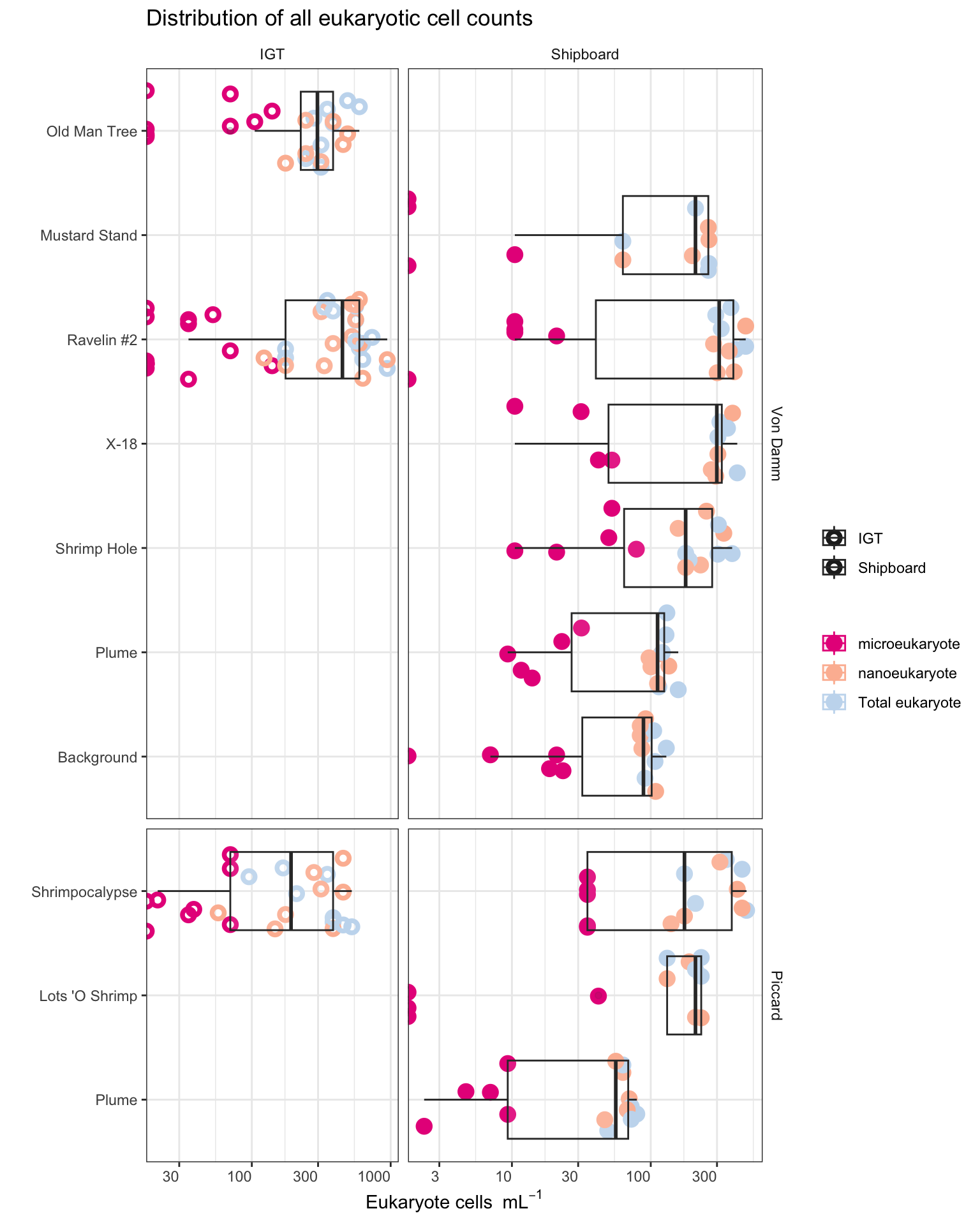

Code

# dev.off()

Eukaryote cell concentration (cells/ml) are lower in the background and plume samples compared to vent sites. ~10s-100 cells/ml in background and plume compared to ~300-1000 cells per ml at the vent sites. These values are also consistent between each vent site (Von Damm and Piccard) and between Bag and IGT samples.

Boxplot represents the median (line in box) and the 1st and 3rd quartiles in the lower and upper hinges, respectively (25th and 75th percentiles). Black data points are outliers from the boxplot. Upper and lower whiskers represent the 1.5 * interquartile ranges. Pink data points are the values contributing to the boxplot (individial counts across replicates and time points.)

eukCONC is the sum of micro and nano. Because there was a discrepency between the micro and nano cell counts, we plan to combine for most of the analysis. Here we show that the cell concentration across replicate samples was similar throughout experiments. And that the bag versus IGT experiment results were within range of one another.

2.2 Plot eukaryote cell concentration over time.

Include plot over time.

Figure S5

Code

# Plot trend line of euk cell count for all experiments
# svg(filename = "../../../Manuscripts_presentations_reviews/MCR-grazing-2023/svg-files-figures/figS4.svg")
counts_cellsml_avg %>%
  mutate(EXP_CATEGORY = case_when(
    EXP_TYPE == "Bag" ~ "Shipboard",
    TRUE ~ "IGT"
  )) %>% 
  mutate(EXP_CATEGORY_WREP = case_when(
    EXP_TYPE == "Bag" ~ "Shipboard",
    TRUE ~ IGT_REP
  )) %>% 
  # Factor name order and label
  mutate(SiteOrder = factor(Site, levels = site_ids, labels = site_fullname)) %>% 
  mutate(NameOrder = factor(Name, levels = vent_ids, labels = vent_fullname)) %>% 
  filter(VARIABLE == "eukCONC") %>%
  unite("Experiment", NameOrder, EXP_CATEGORY, sep = "-", remove = FALSE) %>%
  unite("Experiment_rep", NameOrder, EXP_CATEGORY_WREP, sep = "-", remove = FALSE) %>%
  ggplot(aes(x = TimePoint, y = MEAN, shape = EXP_CATEGORY, fill = NameOrder, 
             color = NameOrder)) +
    geom_path(aes(group = Experiment_rep), color = "black") +
    geom_errorbar(aes(ymax = (MEAN + SEM), ymin = (MEAN - SEM)), width = 0.2) +
    geom_point(stat = "identity", size = 2, stroke = 2, aes(shape = EXP_CATEGORY, 
                                                fill = NameOrder, 
                                                color = NameOrder)) +
    scale_shape_manual(values = c(1, 21)) +
    scale_fill_brewer(palette = "Paired") +
    scale_color_brewer(palette = "Paired") +
    scale_y_log10() +
    facet_wrap(SiteOrder ~ EXP_CATEGORY, scales = "free") +
    theme_classic() + theme(strip.background = element_blank(), 
                            legend.title = element_blank(),
                            title = element_text(size = 7, face = "bold"),
                            axis.title = element_text(size = 9)) +
    labs(title = "Total euk cell counts for each experiment", y = bquote("Average eukaryote cells "~mL^-1), x = "Time point")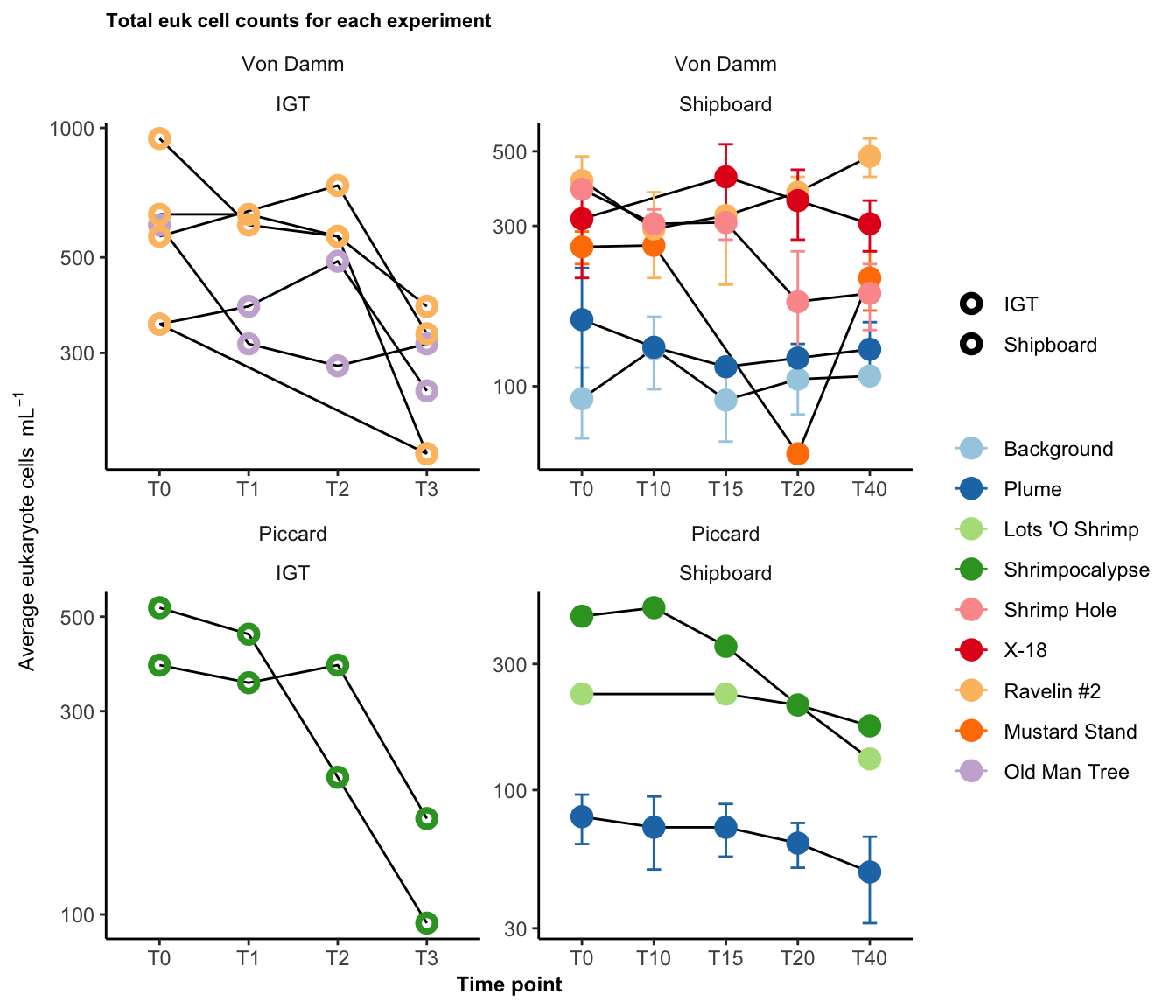

Code

# dev.off()

There is an overall drop in euk cells/ml in the final time point. This is especially true among the IGT samples. We take this into consideration in the manuscript, where the T3 (or final time point) for the IGT experiments is removed.

2.3 Plot T0 only counts for cells/ml plot

For Figure 1, we want to show eukaryote cell abundances. For this value, we will use the total eukaryote cell values (micro + nano) from the initial time points (T0).

Code

# Plot trend line of euk cell count for all experiments
euk_plot <- counts_cellsml_avg %>%
  mutate(EXP_CATEGORY = case_when(
    EXP_TYPE == "Bag" ~ "Shipboard",
    TRUE ~ "IGT"
  )) %>% 
  mutate(EXP_CATEGORY_WREP = case_when(
    EXP_TYPE == "Bag" ~ "Shipboard",
    TRUE ~ IGT_REP
  )) %>% 
  # Factor name order and label
  mutate(SiteOrder = factor(Site, levels = site_ids, labels = site_fullname)) %>% 
  mutate(NameOrder = factor(Name, levels = vent_ids, labels = vent_fullname)) %>% 
  filter(VARIABLE == "eukCONC") %>%
  filter(TimePoint == "T0") %>% 
  filter(!(grepl("b", IGT_REP))) %>% 
  unite("SITE_TYPE", Site, EXP_CATEGORY, sep = "-", remove = FALSE) %>%
  unite("Experiment", Name, EXP_CATEGORY, sep = "-", remove = FALSE) %>%
  unite("Experiment_rep", Name, EXP_CATEGORY_WREP, sep = "-", remove = FALSE) %>%
  ggplot(aes(x = NameOrder, y = MEAN, shape = SITE_TYPE, fill = SITE_TYPE, 
             color = SITE_TYPE)) +
    geom_errorbar(aes(ymax = (MEAN + SEM), ymin = (MEAN - SEM)), width = 0.2, color = "black") +
    geom_point(stat = "identity", size = 2, stroke = 2, aes(shape = SITE_TYPE, 
                                                fill = SITE_TYPE, 
                                                color = SITE_TYPE)) +
    scale_shape_manual(values = c(21, 21, 21, 21)) +
    scale_fill_manual(values = c("white", "#264653", "white", "#E76F51")) +
    scale_color_manual(values = c("#264653", "#264653", "#E76F51", "#E76F51")) +
    scale_y_log10() +
    # cfacet_grid(. ~ SiteOrder, scales = "free") +
    facet_grid(.~SiteOrder, space = "free", scales = "free") +
    theme_minimal() +
    theme(panel.grid.major = element_line(), panel.grid.minor = element_blank(),
           panel.background = element_blank(), 
           axis.line = element_line(colour = "black"), 
           axis.text.x = element_text(color="black", size = 13, 
                                      angle = 45, hjust = 1, vjust = 1), 
           axis.text.y = element_text(color="black", size = 13),
           axis.title =element_text(color="black", size = 13),
           axis.ticks = element_line(),
           strip.text =element_blank(), legend.title = element_blank()) +
  labs(x = "", y = bquote("Eukaryote cells "~mL^-1),
       title = "")

euk_plot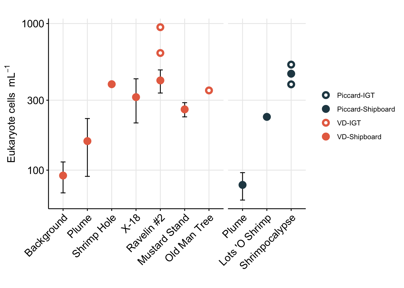

Above Figure shows the eukaryote cell abundances separated by vent site (x-axis).

Boxplot eukaryote cell abundance

To better show comparison across vent fields (Von Damm vs. Piccard), habitat type (vent fluid vs. background or non-vent), and experiment type (shipboard vs. IGT), cell abundances are better shown as a box plot.

Code

# Plot trend line of euk cell count for all experiments
boxplot_eukcell_site <- counts_cellsml_avg %>%
  mutate(LOCATION_BIN = case_when(
    (Name == "Plume") ~ "Non-vent",
    (Name == "BSW") ~ "Non-vent",
    TRUE ~ "Vent"
  )) %>% 
  # Factor name order and label
  mutate(SiteOrder = factor(Site, levels = site_ids, labels = site_fullname)) %>% 
  filter(VARIABLE == "eukCONC") %>%
  filter(TimePoint == "T0") %>% 
  filter(!(grepl("b", IGT_REP))) %>% 
  ggplot(aes(x = LOCATION_BIN, y = MEAN)) +
  geom_boxplot(aes(color = SiteOrder)) +
    geom_jitter(stat = "identity", size = 2, width = 0.3, stroke = 2, shape = 21, aes(fill = SiteOrder,
                                                color = SiteOrder)) +
    scale_fill_manual(values = c("#264653", "#E76F51")) +
    scale_color_manual(values = c("#264653", "#E76F51")) +
    scale_y_log10(position = "right") +
    coord_flip() +
    facet_grid(.~SiteOrder) +
    theme_minimal() +
  theme(panel.grid.major = element_line(), panel.grid.minor = element_blank(),
        panel.background = element_blank(), 
        axis.line = element_line(colour = "black"), 
        axis.text.x = element_text(color="black", size = 10, 
                                   angle = 0, hjust = 0.5, vjust = 0), 
        axis.text.y = element_text(color="black", size = 12),
        axis.title =element_text(color="black", size = 12),
        axis.ticks = element_line(),
        strip.text =element_blank(), legend.title = element_blank()) +
  labs(x = "", y = bquote("Eukaryote cells "~mL^-1),
       title = "")
boxplot_eukcell_site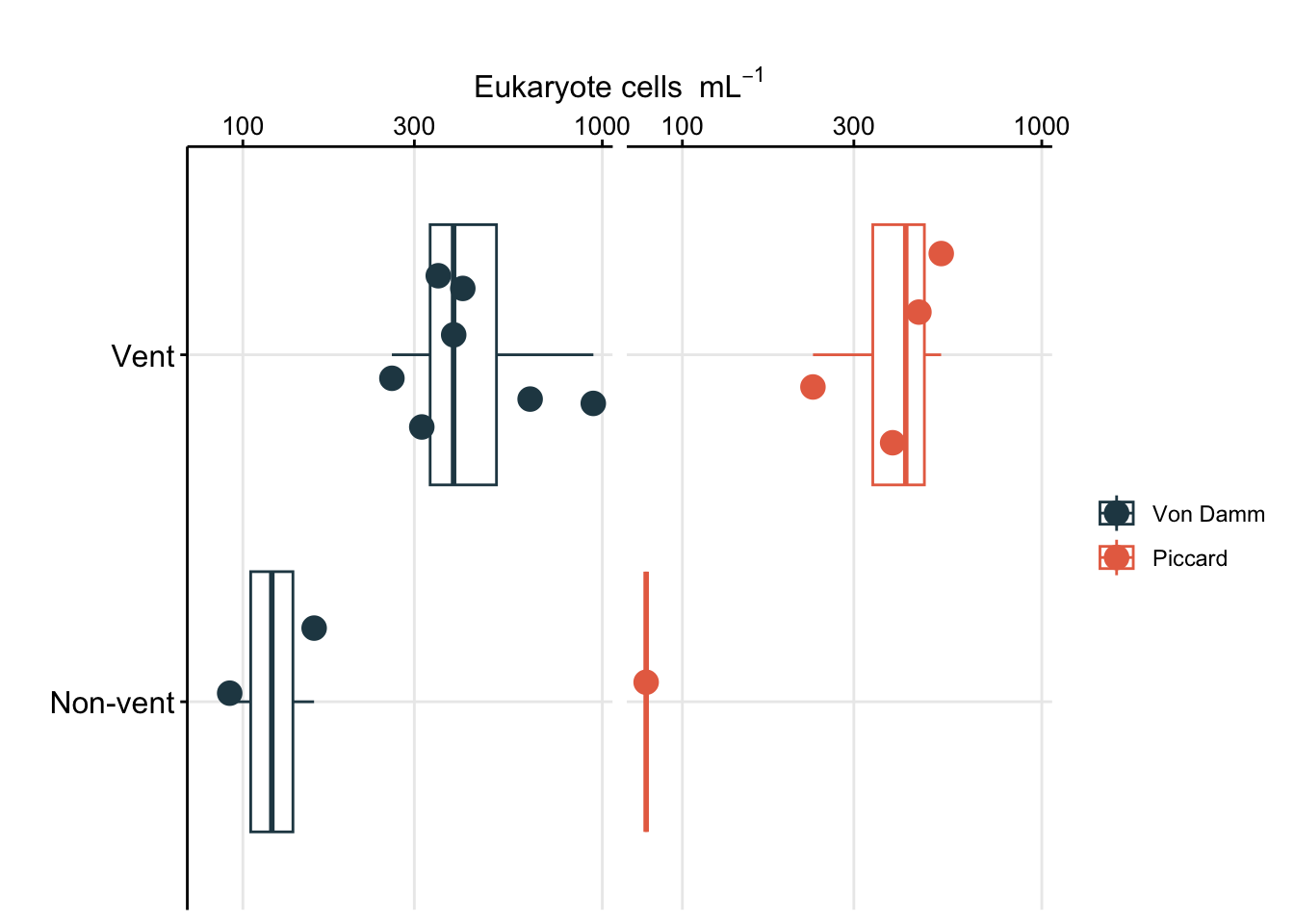

Repeat, but subset vent sites only and group by experiment approach.

Code

# Plot trend line of euk cell count for all experiments
boxplot_eukcell_exp <-counts_cellsml_avg %>%
  mutate(EXP_CATEGORY = case_when(
    EXP_TYPE == "Bag" ~ "Shipboard",
    TRUE ~ "IGT"
  )) %>% 
  mutate(EXP_CATEGORY_WREP = case_when(
    EXP_TYPE == "Bag" ~ "Shipboard",
    TRUE ~ IGT_REP
  )) %>% 
  mutate(LOCATION_BIN = case_when(
    (Name == "Plume") ~ "Non-vent",
    (Name == "BSW") ~ "Non-vent",
    TRUE ~ "Vent"
  )) %>% 
  # Factor name order and label
  mutate(SiteOrder = factor(Site, levels = site_ids, labels = site_fullname)) %>% 
  filter(VARIABLE == "eukCONC") %>%
  filter(LOCATION_BIN == "Vent") %>% 
  filter(TimePoint == "T0") %>% 
  filter(!(grepl("b", IGT_REP))) %>% 
  ggplot(aes(x = EXP_CATEGORY, y = MEAN)) +
  geom_boxplot() +
    geom_jitter(stat = "identity", size = 2, width = 0.3, stroke = 2, aes(shape = EXP_CATEGORY)) +
    scale_shape_manual(values = c(21, 19)) +  
  # scale_fill_manual(values = c("#264653", "#E76F51")) +
    # scale_color_manual(values = c("#264653", "#E76F51")) +
    scale_y_log10(position = "right") +
    coord_flip() +
    # facet_grid(.~SiteOrder) +
    theme_minimal() +
    theme(panel.grid.major = element_line(), panel.grid.minor = element_blank(),
           panel.background = element_blank(), 
           axis.line = element_line(colour = "black"), 
           axis.text.x = element_text(color="black", size = 10, 
                                      angle = 0, hjust = 0.5, vjust = 0), 
           axis.text.y = element_text(color="black", size = 12),
           axis.title =element_text(color="black", size = 12),
           axis.ticks = element_line(),
           strip.text =element_blank(), legend.title = element_blank()) +
  labs(x = "", y = bquote("Eukaryote cells "~mL^-1),
       title = "")
boxplot_eukcell_exp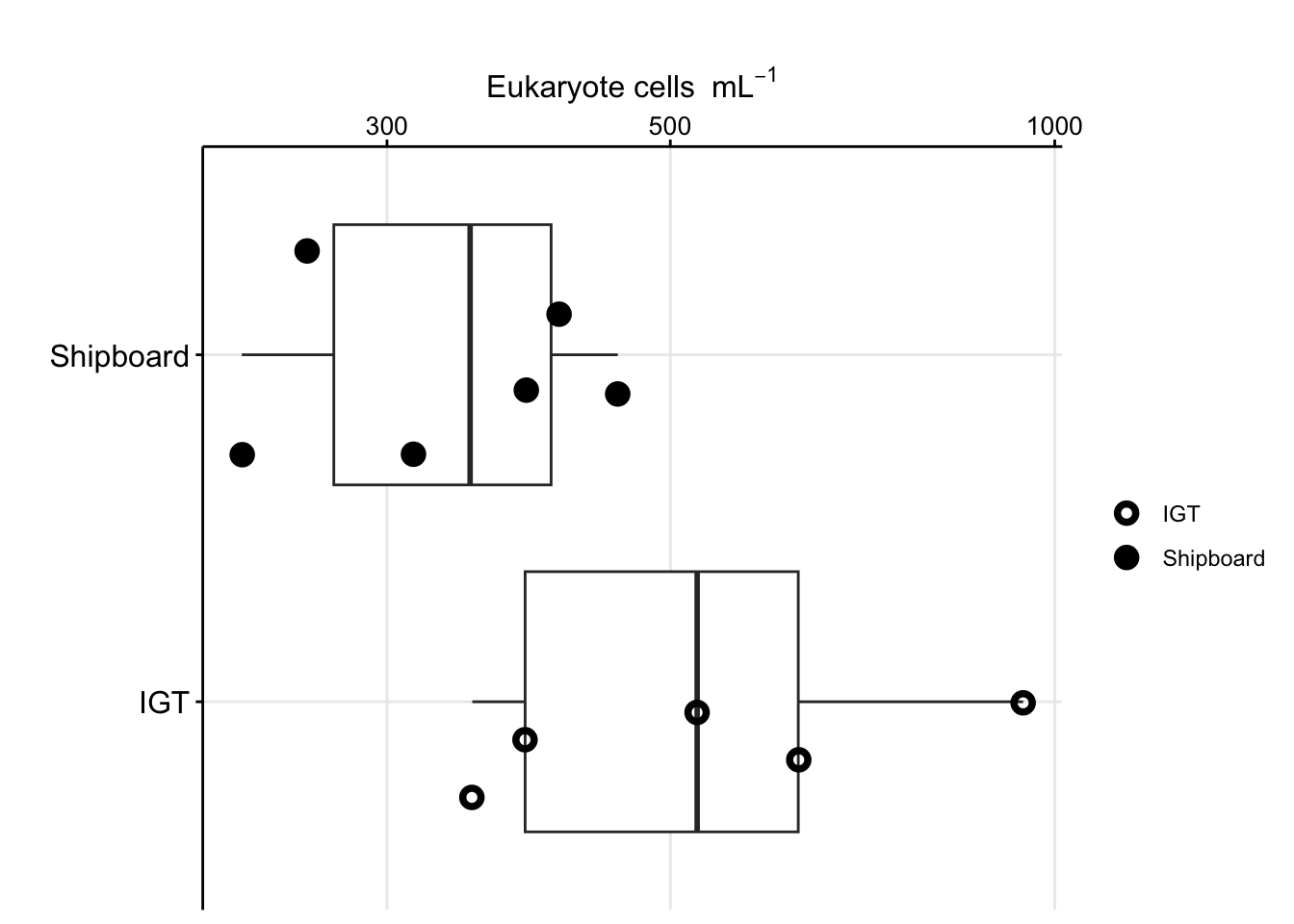

Option to show eukaryote cell abundances without a log scale.

Code

counts_cellsml_all %>%
  filter(TimePoint == "T0") %>% 
  mutate(EXP_CATEGORY = case_when(
    grepl("IGT", EXPID) ~ "IGT",
    TRUE ~ "Shipboard"
  )) %>%
  mutate(TYPE_BIN = case_when(
    Name == "Plume" ~ "Non-vent",
    Name == "Background" ~ "Non-vent",
    TRUE ~ "Vent"
  )) %>% 
  mutate(SITE_TYPE = case_when(
    grepl("IGT", EXPID) ~ paste(Site, "IGT"),
    TRUE ~ paste(Site, "Shipboard"),
  )) %>% 
  # unite("SITE_TYPE", Site, EXP_CATEGORY, sep = "-", remove = FALSE) %>%
  # Factor name order and label
  mutate(SiteOrder = factor(Site, levels = site_ids, labels = site_fullname)) %>% 
  mutate(NameOrder = factor(Name, levels = vent_ids, labels = vent_fullname)) %>% 
  filter(!(grepl("b", EXPID))) %>% 
  ggplot(aes(y = eukCONC, x = TYPE_BIN)) +
    geom_boxplot() +
    geom_jitter(stat = "identity", size = 2, stroke = 2, aes(shape = SITE_TYPE, 
                                                fill = SITE_TYPE, 
                                                color = SITE_TYPE)) +
    scale_shape_manual(values = c(21, 21, 21, 21)) +
    scale_fill_manual(values = c("white", "#264653", "white", "#E76F51")) +
    scale_color_manual(values = c("#264653", "#264653", "#E76F51", "#E76F51")) +
    theme_minimal() +
    theme(panel.grid.major = element_line(), panel.grid.minor = element_blank(),
           panel.background = element_blank(), 
           axis.line = element_line(colour = "black"), 
           axis.text.x = element_text(color="black", size = 13, 
                                      angle = 45, hjust = 1, vjust = 1), 
           axis.text.y = element_text(color="black", size = 13),
           axis.title =element_text(color="black", size = 13),
           axis.ticks = element_line(),
           strip.text =element_blank(), legend.title = element_blank()) +
  labs(x = "", y = bquote("Eukaryote cells "~mL^-1),
       title = "")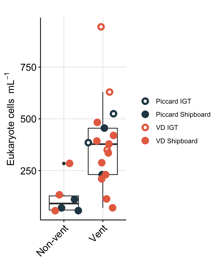

Code

# save(counts_cellsml_all, counts_cellsml_avg, counts_occur, file = "output-data/MCR-cellcount-dfs.RData")

3 Bacteria & archaea cell counts

DAPI slide counts from prokaryotes from same sites. Import and compare.

Code

prok <- read.delim("input-data/prokINSITU-counts-compiled.txt")

insitu_proks <- prok %>% 
  filter(CELLML != "not countable") %>% 
  separate(SAMPLE, c("Site", "Name"), sep = "-", remove = FALSE) %>% 
  group_by(SAMPLE, Site, Name) %>% 
  summarise(MEAN = mean(as.numeric(CELLML)),
            SD = sd(CELLML),
            SEM = (sd(CELLML)/sqrt(length(CELLML))),
            MIN = min(CELLML),
            MAX = max(CELLML),
            .groups = "rowwise") %>% 
  data.frame

3.1 Cells per ml (prok)

Visualize counts from proks. Get summary of prok counts, and incorporate into plot. Throughout dataset, sample called “Quakeplume” did not work. This was an opportunistic sample that can be removed.

Code

insitu_proks %>% filter(Name != "Quakeplume") %>% 
  mutate(type = case_when(
  Name == "BSW" ~ "non-vent",
  Name == "Plume" ~ "non-vent",
  TRUE ~ "vent"
)) %>% 
  group_by(type, Site) %>% 
      summarize(mean = mean(MEAN),
            min = min(MEAN),
            max = max(MEAN))

`summarise()` has grouped output by 'type'. You can override using the
`.groups` argument.

# A tibble: 4 × 5
# Groups:   type [2]
  type     Site       mean    min     max
  <chr>    <chr>     <dbl>  <dbl>   <dbl>
1 non-vent Piccard  31645. 11860.  51429.
2 non-vent VD       27184. 16478.  37890.
3 vent     Piccard 109713. 53878. 238586.
4 vent     VD       40907.  8816. 111430.

Factor site names, so order can be uniform with other figures.

Code

# Ordered by temperature
insitu_proks$Name_order <- factor(insitu_proks$Name, levels = c("BSW", "Plume",
                                                                "ShrimpHole", "X18", "MustardStand", 
                                                                "Rav2", "OMT","Bartizan","ArrowLoop", "Rav1",
                                                                "Quakeplume", "LotsOShrimp", "SouthofHotChimlet",
                                                                "SouthofLungSnack", "Shrimpocalypse", "ShrimpGulley", 
                                                                "HotChimlet1"), 
                                  labels = c("Background","Plume", 
                                             "Shrimp Hole", "X-18","Mustard Stand",
                                             "Ravelin #2", "Old Man Tree", "Bartizan", "Arrow Loop", "Ravelin #1",
                                          
                                             "Quakeplume", "Lots 'O Shrimp", "South of Hot Chimlet", 
                                             "South of LungSnack", "Shrimpocalypse", "Shrimp Gulley", "Hot Chimlet #1"))

site_ids <- c("VD", "Piccard")
site_fullname <- c("Von Damm", "Piccard")
insitu_proks$Site_order <- factor(insitu_proks$Site, levels = site_ids, labels = site_fullname)
site_color <- c("#E76F51", "#264653")
site_fill <- c("#E76F51", "#264653")
# names(site_color) <- site_fullname

Write function to output scientific notation in the plot with x 10^a

Code

library(scales)

Attaching package: 'scales'

The following object is masked from 'package:purrr':

    discard

The following object is masked from 'package:readr':

    col_factor

Code

scientific_10 = function(x) {
  ifelse(
    x==0, "0",
    parse(text = sub("e[+]?", " %*% 10^", scales::scientific_format()(x)))
  )
} 

Code

prok_plot <- ggplot(insitu_proks, aes(x = Name_order, y = MEAN)) +
  geom_errorbar(aes(ymax = (MEAN + SEM), ymin = (MEAN - SEM)), width = 0.2) +
  geom_point(stat = "identity", shape = 21, stroke = 2, aes(fill = Site_order,
                                                            color = Site_order), size = 3) +
  facet_grid(.~ Site_order, space = "free", scales = "free") +
  scale_fill_manual(values = c("#E76F51", "#264653")) +
  scale_color_manual(values = c("#E76F51", "#264653")) +
  labs(y = bquote("Prokaryote cells "~mL^-1), x = "", title = "") +
  scale_y_log10(label = scientific_10) +
  # scale_y_log10(label=trans_format("log10",math_format(10^.x))) +
  # scale_y_continuous(label = scientific_10) +
  theme_minimal() +
    theme(panel.grid.major = element_line(), panel.grid.minor = element_blank(),
           panel.background = element_blank(), 
           axis.line = element_line(colour = "black"), 
           axis.text.x = element_text(color="black", size = 13, 
                                      angle = 45, hjust = 1, vjust = 1), 
           axis.text.y = element_text(color="black", size = 13),
           axis.title =element_text(color="black", size = 13),
           axis.ticks = element_line(),
           strip.text =element_blank(), legend.title = element_blank())
prok_plot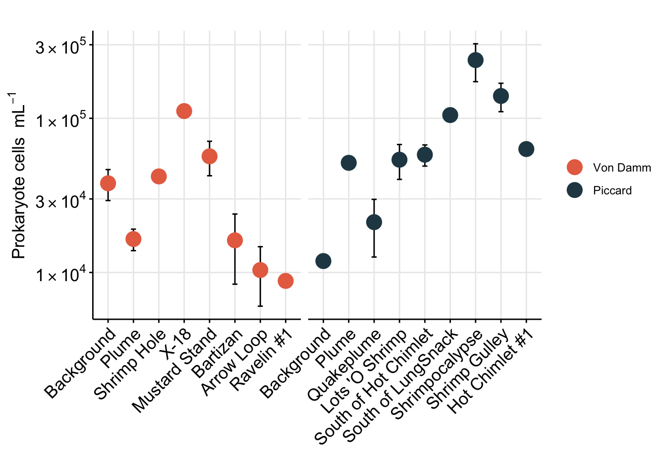

Show prokaryote cell abundance as boxplot.

Code

insitu_proks %>% 
  mutate(TYPE_BIN = case_when(
    Name == "BSW" ~ "Non-vent",
    Name == "Plume" ~ "Non-vent",
    TRUE ~ "Vent"
  )) %>% 
ggplot(aes(x = TYPE_BIN, y = MEAN)) +
  # geom_errorbar(aes(ymax = (MEAN + SEM), ymin = (MEAN - SEM)), width = 0.2) +
  geom_boxplot() +
  geom_jitter(stat = "identity", shape = 21, stroke = 2, aes(fill = Site_order,
                                                            color = Site_order), size = 3) +
  scale_fill_manual(values = c("#E76F51", "#264653")) +
  scale_color_manual(values = c("#E76F51", "#264653")) +
  labs(y = bquote("Prokaryote cells "~mL^-1), x = "", title = "") +
  scale_y_log10(label = scientific_10) +
  # scale_y_log10(label=trans_format("log10",math_format(10^.x))) +
  # scale_y_continuous(label = scientific_10) +
  theme_minimal() +
    theme(panel.grid.major = element_line(), panel.grid.minor = element_blank(),
           panel.background = element_blank(), 
           axis.line = element_line(colour = "black"), 
           axis.text.x = element_text(color="black", size = 13, 
                                      angle = 45, hjust = 1, vjust = 1), 
           axis.text.y = element_text(color="black", size = 13),
           axis.title =element_text(color="black", size = 13),
           axis.ticks = element_line(),
           strip.text =element_blank(), legend.title = element_blank())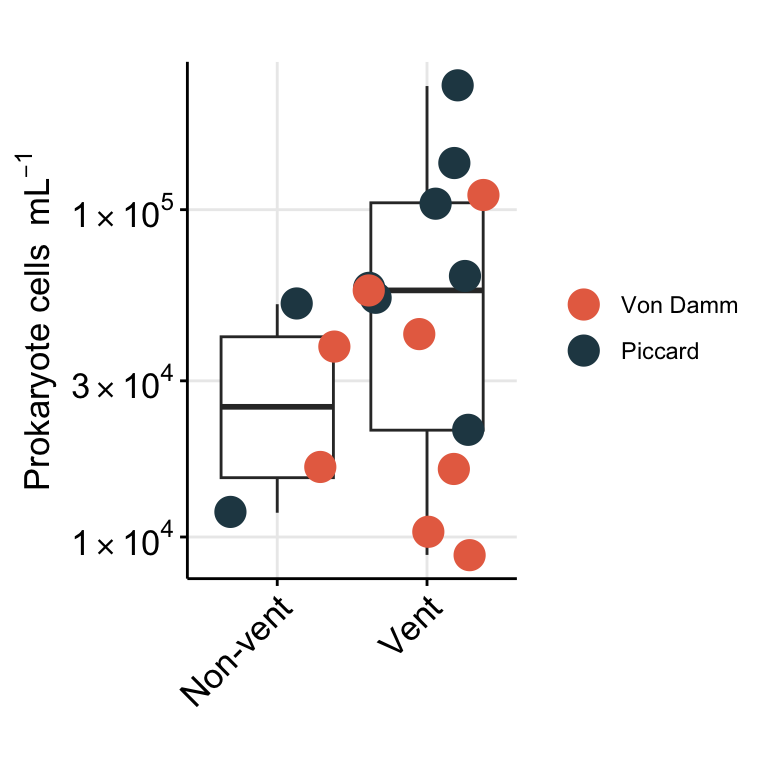

Compare euk and prok cell abundance

Combined eukaryote and prokaryote cell counts.

Code

euk_prok_ab <- (euk_plot + theme(legend.position = "top")) + (prok_plot + theme(legend.position = "top")) + patchwork::plot_layout(ncol = 2) + patchwork::plot_annotation(tag_levels = "a")
euk_prok_ab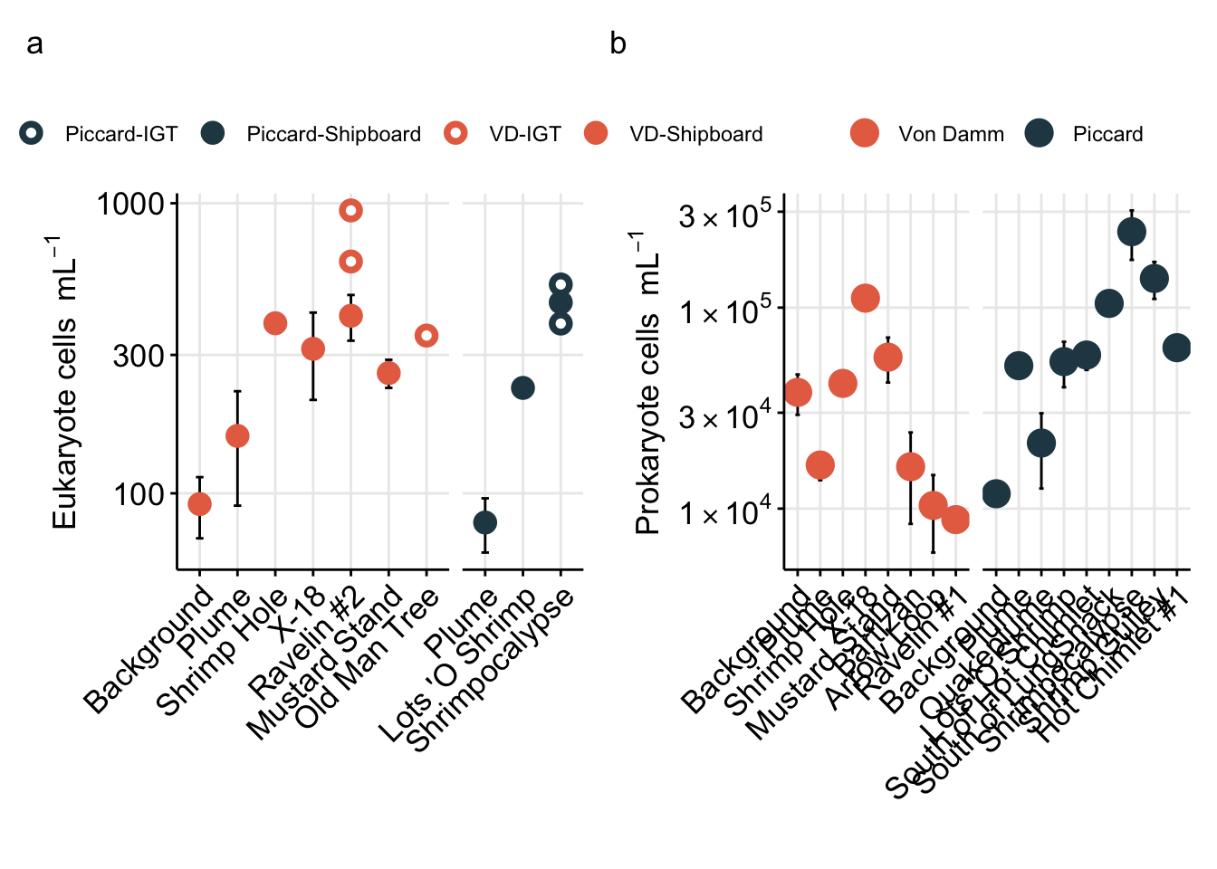

Combine with previous MCR cell counts

Compare in situ prokaryote cell counts from 2020 to previous years

Code

prok_prev <- read.csv("input-data/cellcount_previousyr.csv")

prok_prev_formatted <- prok_prev %>% 
  mutate(VENTSITE = case_when(
    grepl("Piccard", Site) ~ "Piccard",
    grepl("Von Damm", Site) ~ "VD"
  )) %>% 
  filter(!is.na(YEAR)) %>% #QC of 
  # filter(cells_ml != "NC") %>% 
  # filter(cells_ml != "") %>% 
  # filter(cells_ml != "no data") %>% 
  type.convert(as.is = TRUE, numerals = "no.loss") %>%
  select(YEAR, VENTSITE, NAME = Name, REP=Replicate, CELLML = cells_ml, ORIGSAMPLE = Orig_vent_site_ID, ID_number, Origin)

Re-import 2020 data to compare.

Code

# Re-import 2020
prok <- read.delim("input-data/prokINSITU-counts-compiled.txt")
proks_allyrs <- prok %>% 
  separate(SAMPLE, c("VENTSITE", "NAME"), sep = "-", remove = FALSE) %>% 
  mutate(YEAR = 2020) %>%
  select(YEAR, VENTSITE, NAME, REP, CELLML, ORIGSAMPLE = BAC) %>% 
  bind_rows(prok_prev_formatted %>% select(-ID_number, -Origin)) %>% 
  type.convert(as.is = TRUE) %>%
  # Remove not countable or not data samples:
  filter(CELLML != "NC") %>%
  filter(CELLML != "") %>%
  filter(CELLML != "no data") %>%
  filter(CELLML != "not countable") %>% 
  data.frame

vent_order <- c("BSW","Plume","Quakeplume","NearsummitBeebee","MainOrifice","NearMainOrifice","Rav1","HotChimlet1","HotChimlet","SouthofHotChimlet","NearHotChimlet","HotCracks1","HotCracks2","ShrimpHole","ShrimpHole(X18)","X18","X19","SouthofLungSnack","TwinPeaks","OMT","WhiteCastle","GingerCastle","ArrowLoop","Bartizan","LotsOShrimp","MustardStand","ShrimpButtery","ShrimpCanyon","ShrimpGulley","Shrimpocalypse","ShrimpVegas")
vent_names <- c("Background","Plume","Quakeplume","Near summit Beebee Vents Mound","Main Orifice","Near Main Orifice","Ravelin #1","Hot Chimlet #1","Hot Chimlet","South of Hot Chimlet","Near Hot Chimlet","Hot Cracks #1","Hot Cracks #2","Shrimp Hole","Shrimp Hole (X-18)","X-18","X-19","South of Lung Snack","Twin Peaks","Old Man Tree","White Castle","Ginger Castle","Arrow Loop","Bartizan","Lots O Shrimp","Mustard Stand","Shrimp Buttery","Shrimp Canyon","Shrimp Gulley","Shrimpocalypse","Shrimp Vegas")
proks_allyrs$NAME_ORDER <- factor(proks_allyrs$NAME, levels = vent_order, labels = vent_names)
proks_allyrs$VENTSITE_ORDER <- factor(proks_allyrs$VENTSITE, levels = c("Piccard", "VD"), labels = c("Piccard", "Von Damm"))

Plot by year.

Code

# pdf("compare-across-yr-cellcount-04052021.pdf", h = 8, w = 7)
ggplot(proks_allyrs, aes(x = NAME_ORDER, y = as.numeric(CELLML), fill = factor(YEAR), shape = VENTSITE_ORDER)) +
  geom_point(stat = "identity", aes(fill = factor(YEAR)), size = 3) +
  scale_shape_manual(values = c(21,23)) +
  coord_flip() +
  facet_grid(VENTSITE_ORDER ~ ., space = "free", scales = "free") +
  scale_y_log10() +
  scale_fill_manual(values = c("#1c9099", "#ffeda0", "#fc4e2a")) +
  theme_linedraw() +
  theme(axis.text = element_text(color = "black", size = 10),
        strip.background = element_blank(),
        strip.text.y = element_text(color = "black", size = 11, hjust = 0, vjust = 1),
        legend.title = element_blank(),
        legend.position = "bottom",
        panel.grid.minor = element_blank(),
        panel.grid.major = element_line(color = "grey")) +
  labs(y = bquote("Cells "~mL^-1), x = "") +
  guides(fill=guide_legend(override.aes=list(shape=22)))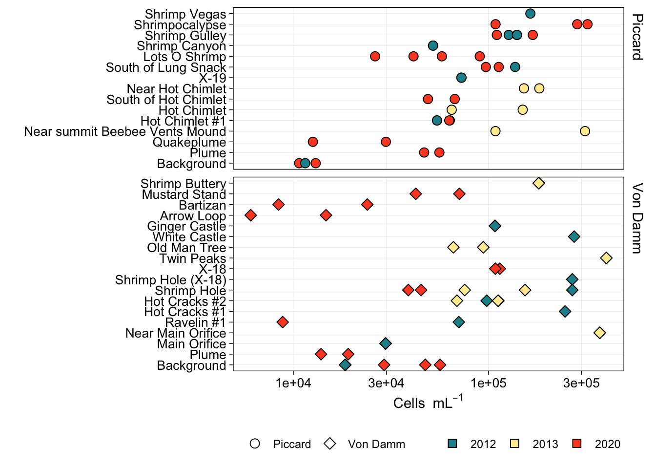

Code

# dev.off()

Code

# head(insitu_proks)
# names(counts_cellsml_avg)
prok_tojoin <- insitu_proks %>% 
  mutate(MEAN_SIG = signif(as.numeric(MEAN), digits = 5),
         MIN_sig = signif(as.numeric(MIN), digits = 4),
         MAX_sig = signif(as.numeric(MAX), digits = 4)) %>% 
  unite("PROK_MinMax", MIN_sig, MAX_sig, sep = " / ") %>%
  select(Site, Name, PROK_ml = MEAN_SIG, PROK_MinMax, PROK_sem = SEM)
# prok_tojoin

3.2 Compile table with euk and prok counts

Part of Table 1.

Code

euk_prok_counts <- counts_cellsml_avg %>%
  mutate(EXP_CATEGORY = case_when(
    EXP_TYPE == "Bag" ~ "Shipboard",
    TRUE ~ "IGT"
  )) %>% 
  mutate(EXP_CATEGORY_WREP = case_when(
    EXP_TYPE == "Bag" ~ "Shipboard",
    TRUE ~ IGT_REP
  )) %>% 
  # Factor name order and label
  mutate(SiteOrder = factor(Site, levels = site_ids, labels = site_fullname)) %>% 
  mutate(NameOrder = factor(Name, levels = vent_ids, labels = vent_fullname)) %>% 
  filter(VARIABLE == "eukCONC") %>%
  filter(TimePoint == "T0") %>% 
  filter(!(grepl("b", IGT_REP))) %>% 
  unite("SITE_TYPE", Site, EXP_CATEGORY, sep = "-", remove = FALSE) %>%
  unite("Experiment", Name, EXP_CATEGORY, sep = "-", remove = FALSE) %>%
  unite("Experiment_rep", Name, EXP_CATEGORY_WREP, sep = "-", remove = FALSE) %>% 
  mutate(MEAN_SIG = signif(MEAN, digits = 5),
         MIN_sig = signif(MIN, digits = 4),
         MAX_sig = signif(MAX, digits = 4)) %>% 
  unite("EUK_MinMax", MIN_sig, MAX_sig, sep = " / ") %>% 
  select(Site, Name, SITE_TYPE, Experiment, Experiment_rep, VARIABLE, EUK_ml = MEAN_SIG, EUK_MinMax, EUK_sem = SEM) %>% 
  left_join(prok_tojoin)

Joining with `by = join_by(Site, Name)`

Code

euk_prok_counts # add to this later for Table 1

      Site           Name         SITE_TYPE               Experiment
1  Piccard    LotsOShrimp Piccard-Shipboard    LotsOShrimp-Shipboard
2  Piccard          Plume Piccard-Shipboard          Plume-Shipboard
3  Piccard Shrimpocalypse Piccard-Shipboard Shrimpocalypse-Shipboard
4  Piccard Shrimpocalypse       Piccard-IGT       Shrimpocalypse-IGT
5  Piccard Shrimpocalypse       Piccard-IGT       Shrimpocalypse-IGT
6       VD            BSW      VD-Shipboard            BSW-Shipboard
7       VD   MustardStand      VD-Shipboard   MustardStand-Shipboard
8       VD            OMT            VD-IGT                  OMT-IGT
9       VD          Plume      VD-Shipboard          Plume-Shipboard
10      VD           Rav2      VD-Shipboard           Rav2-Shipboard
11      VD           Rav2            VD-IGT                 Rav2-IGT
12      VD           Rav2            VD-IGT                 Rav2-IGT
13      VD     ShrimpHole      VD-Shipboard     ShrimpHole-Shipboard
14      VD            X18      VD-Shipboard            X18-Shipboard
             Experiment_rep VARIABLE  EUK_ml    EUK_MinMax    EUK_sem PROK_ml
1     LotsOShrimp-Shipboard  eukCONC 230.910 230.9 / 230.9         NA   53878
2           Plume-Shipboard  eukCONC  79.301   55.98 / 112  16.819081   51429
3  Shrimpocalypse-Shipboard  eukCONC 454.820 454.8 / 454.8         NA  238590
4       Shrimpocalypse-IGT3  eukCONC 384.840 384.8 / 384.8         NA  238590
5       Shrimpocalypse-IGT7  eukCONC 524.790 524.8 / 524.8         NA  238590
6             BSW-Shipboard  eukCONC  91.838 69.97 / 113.7  21.866127   37890
7    MustardStand-Shipboard  eukCONC 259.770 230.9 / 288.6  28.863287   56677
8                  OMT-IGT4  eukCONC 349.860 349.9 / 349.9         NA      NA
9           Plume-Shipboard  eukCONC 157.770 55.98 / 284.4  67.098589   16478
10           Rav2-Shipboard  eukCONC 409.330 335.9 / 482.8  73.470185      NA
11                Rav2-IGT4  eukCONC 944.620 944.6 / 944.6         NA      NA
12                Rav2-IGT5  eukCONC 629.740 629.7 / 629.7         NA      NA
13     ShrimpHole-Shipboard  eukCONC 385.720 377.8 / 393.6   7.871806   41983
14            X18-Shipboard  eukCONC 314.870 209.9 / 419.8 104.957407  111430
       PROK_MinMax  PROK_sem
1    26240 / 90260 13727.191
2    46810 / 56050  4618.126
3  108700 / 322000 65792.588
4  108700 / 322000 65792.588
5  108700 / 322000 65792.588
6    18470 / 56470  8608.427
7    42400 / 70950 14274.207
8             <NA>        NA
9    13850 / 19100  2623.935
10            <NA>        NA
11            <NA>        NA
12            <NA>        NA
13   38830 / 45130  3148.722
14 108500 / 114400  2973.793

4 Estimate grazing effect

Calculate FLP per eukaryotic cell over time. Goal is to make these calculations and then determine best fit line. Slope of best fit line is the grazing rate. Need to take into account euk cells with FLPs and then the euk cells withOUT FLPs, these will be zeroes to take into account for FLPs/euk averages.

Code

load("output-data/MCR-cellcount-dfs.RData", verbose = TRUE)

Loading objects:
  counts_cellsml_all
  counts_cellsml_avg
  counts_occur

4.1 Determine FLP per euk cell

Isolate euk cell counts with FLPs (comma separated for counts). These need to be separated into rows, use counts_occur data frame from above. We can use the command separate_rows() to do this.

Code

# Select nano and micro counts with FLPs
counts_sepflp <- counts_occur %>% 
  filter(!NOTES == "Discard") %>% # uncountable
  filter(!(NOTES == "DTAF stain prevented counts of FLP, Euks only")) %>% # uncountable
  select(DATE, SAMPLE, EXPID, VOL, MAG, FOV, nanoFLP, microFLP) %>%
  # Inputs that are comma separated will be split into a new row
  separate_rows(microFLP, sep = ",", convert = TRUE) %>%
  separate_rows(nanoFLP, sep = ",", convert = TRUE) %>%
  # Replace NAs with zeroes
  replace_na(list(microFLP = 0, nanoFLP = 0)) %>% 
  data.frame

optional gut check of data table modification

Code

# See FOV 23, where nanoFLP is 4,5
# View(counts_occur %>%
# filter(SAMPLE == "VD-Rav2" & EXPID == "T10-Rep1"))

## Check FOV 23. It is separated into 2 rows, 4 and then 5.
# View(counts_sepflp %>%
# filter(SAMPLE == "VD-Rav2" & EXPID == "T10-Rep1"))

Isolate counts that are >0, so only eukaryote cells that were observed to have FLPs are included. Then calculate FLP per euk cell by dividing by 1. Each row is a euk cell, based on data transformation above.

Code

counts_flp <- counts_sepflp %>%
  select(SAMPLE, EXPID, nano_size = nanoFLP, micro_size = microFLP) %>%
  pivot_longer(cols = ends_with("_size"), names_to = "SizeFrac", values_to = "num_of_FLP") %>%
  filter(num_of_FLP > 0) %>%
  separate(SAMPLE, c("Site", "Name"), sep = "-", remove = FALSE) %>%
  separate(EXPID, c("TimePoint", "Replicate"), sep = "-", remove = FALSE) %>%
  mutate(EXP_TYPE = case_when(
    grepl("IGT", Replicate) ~ "IGT",
    grepl("Rep", Replicate) ~ "Bag"
  )) %>%
  mutate(IGT_REP = case_when(
    EXP_TYPE == "IGT" ~ Replicate,
    EXP_TYPE == "Bag" ~ "Bag")) %>%
  group_by(SAMPLE, EXPID, EXP_TYPE, IGT_REP, SizeFrac) %>%
  summarise(total_FLP = sum(num_of_FLP),
            total_euks_wflp = n(),
            .groups = "rowwise") %>%
  data.frame

glimpse(counts_flp)

Rows: 157
Columns: 7
$ SAMPLE          <chr> "Piccard-LotsOShrimp", "Piccard-LotsOShrimp", "Piccard…
$ EXPID           <chr> "T0-Rep3", "T15-Rep3", "T15-Rep3", "T20-Rep3", "T0-Rep…
$ EXP_TYPE        <chr> "Bag", "Bag", "Bag", "Bag", "Bag", "Bag", "Bag", "Bag"…
$ IGT_REP         <chr> "Bag", "Bag", "Bag", "Bag", "Bag", "Bag", "Bag", "Bag"…
$ SizeFrac        <chr> "nano_size", "micro_size", "nano_size", "nano_size", "…
$ total_FLP       <int> 3, 1, 3, 2, 2, 4, 3, 2, 8, 6, 3, 3, 9, 1, 7, 4, 7, 8, …
$ total_euks_wflp <int> 2, 1, 2, 1, 1, 3, 2, 1, 5, 5, 2, 1, 4, 1, 3, 1, 4, 2, …

OUTPUT COLUMNS: (1) total_FLP = sum of FLPs found inside a euk cell (2) total_euks_wflp = number of euks counted with ingested FLP

Repeat above operation for euk cells without any FLP. Here, subset total number of observations where there was a euk cell without FLP. These need to be counted as euk cell without an FLP.

Below code repeats process and compiles with other FLP/euk cell data.

Repeat above process for euk cells without FLPs (0 FLP per euk cell needs to be included in overall average).

Code

counts_flp_compiled <- counts_occur %>% 
  filter(!(NOTES == "Discard")) %>% #Discard bad counts
  filter(!(NOTES == "DTAF stain prevented counts of FLP, Euks only")) %>%
  type.convert(as.is = TRUE) %>% #modify str() for columns
  select(SAMPLE, EXPID, nano_size = nanoNoFLP, micro_size = microNoFLP) %>% #select non flp
  pivot_longer(cols = ends_with("_size"), names_to = "SizeFrac", values_to = "num_of_euks") %>%
  separate(SAMPLE, c("Site", "Name"), sep = "-", remove = FALSE) %>%
  separate(EXPID, c("TimePoint", "Replicate"), sep = "-", remove = FALSE) %>%
  mutate(EXP_TYPE = case_when(
    grepl("IGT", Replicate) ~ "IGT",
    grepl("Rep", Replicate) ~ "Bag"
  )) %>%
  mutate(IGT_REP = case_when(
    EXP_TYPE == "IGT" ~ Replicate,
    EXP_TYPE == "Bag" ~ "Bag")) %>% 
  # filter(num_of_euks > 0) %>% # Remove observed zero counts
  group_by(SAMPLE, EXPID, EXP_TYPE, IGT_REP, SizeFrac) %>%
  summarise(total_euks_noFLP = sum(num_of_euks),
            .groups = "rowwise") %>%
  # Join with FLP count information
  ## SAMPLE, EXPID, EXPTYPE, IGTREP, and SizeFrac variables should match
  left_join(counts_flp) %>% # Join with the counts of FLP per euk cell
  replace_na(list(total_FLP = 0, total_euks_wflp = 0)) %>% #Replace NAs with zero
  data.frame

Joining with `by = join_by(SAMPLE, EXPID, EXP_TYPE, IGT_REP, SizeFrac)`

Code

counts_flp_compiled_all <- counts_flp_compiled %>% 
  # Exclude size fraction:
  group_by(SAMPLE, EXPID, EXP_TYPE, IGT_REP) %>%
  summarise(total_euks_noFLP = sum(total_euks_noFLP),
            total_FLP = sum(total_FLP), 
            total_euks_wflp = sum(total_euks_wflp),
            .groups = "rowwise") %>% 
  add_column(SizeFrac = "total_euks") %>% #Add SizeFrac column
  bind_rows(counts_flp_compiled) %>% # Combine back with flp compiled list
  data.frame

glimpse(counts_flp_compiled_all)

Rows: 336
Columns: 8
$ SAMPLE           <chr> "Piccard-LotsOShrimp", "Piccard-LotsOShrimp", "Piccar…
$ EXPID            <chr> "T0-Rep3", "T15-Rep3", "T20-Rep3", "T40-Rep3", "T0-Re…
$ EXP_TYPE         <chr> "Bag", "Bag", "Bag", "Bag", "Bag", "Bag", "Bag", "Bag…
$ IGT_REP          <chr> "Bag", "Bag", "Bag", "Bag", "Bag", "Bag", "Bag", "Bag…
$ total_euks_noFLP <int> 9, 8, 9, 5, 6, 5, 11, 8, 2, 9, 10, 1, 5, 5, 3, 7, 5, …
$ total_FLP        <int> 3, 4, 2, 0, 6, 5, 8, 6, 3, 12, 8, 11, 19, 5, 4, 9, 11…
$ total_euks_wflp  <int> 2, 3, 1, 0, 4, 3, 5, 5, 2, 5, 4, 5, 6, 4, 3, 5, 4, 1,…
$ SizeFrac         <chr> "total_euks", "total_euks", "total_euks", "total_euks…

The code above takes the processed microscopy counts, and estimates the total number of FLP and the total number of eukaryotes counted (with or without FLP inside). To calculate the rate that FLP were ingested, we need the slope of the line when we plot the number of ingested FLP per eukaryote cell by experiment time.

We will use this equation below: FLPperEuk = total_FLP/(sum(total_euks_noFLP, total_euks_wflp)).

First need to import and compile with metadata to get exact timing of experiments.

Code

metadata <- read.delim("input-data/flp-exp-metadata-compiled.txt")
exp_metadata <- read.csv("input-data/flp_exp_metadata.csv")

Consider IGT replicates.

IGT_#_ denotes a separate IGT experiment. Due to bottle effects and the need to look at how replicate experiments compared, lets keep these separate. For IGT experiments labeled “b”, this means the OTHER HALF of the filter was counted or re-counted as a way to confirm my eukaryote cell counting was precise (explored in manuscript supplement).

Code

counts_flp_calcs_all <- counts_flp_compiled_all %>% 
  # Add in metadata
  # IGTXb are replicate counts, use this to include them as replicates
  separate(EXPID, c("TimePoint", "REP"), sep = "-", remove = FALSE) %>% 
  mutate(
    REP = ifelse(grepl("IGT5b", REP), "IGT5", REP),
    REP = ifelse(grepl("IGT4b", REP), "IGT4", REP),
    REP = ifelse(grepl("Bag", EXP_TYPE), "Bag", REP)) %>% 
  left_join(metadata, by = c("SAMPLE" = "SAMPLE", "TimePoint" = "TimePoint", "REP" = "REP")) %>% 
  left_join(exp_metadata, by = c("SAMPLE" = "SAMPLE", "REP" = "REP")) %>% 
  separate(SAMPLE, c("Site", "Name"), sep = "-", remove = FALSE) %>%
  separate(EXPID, c("TimePoint", "Replicate_ID"), sep = "-", remove = FALSE) %>%
  ## Treat repeated IGT counts completely separate
  group_by(SAMPLE, Site, Name, EXPID, TimePoint, Replicate_ID, EXP_TYPE, IGT_REP, SizeFrac) %>%
  ## Treat repeated IGT counts as replicates (e.g., IGT4b and IGT4 == IGT4)
  # group_by(SAMPLE, Site, Name, EXPID, TimePoint, Replicate_ID, EXP_TYPE, REP, SizeFrac) %>%
  # FLPperEuk is the total FLP divided by the total number of euk cells counted
  mutate(FLPperEuk = total_FLP/(sum(total_euks_noFLP, total_euks_wflp))) %>%
  unite("Experiment", Name, REP, sep = "-", remove = FALSE) %>%
  data.frame

glimpse(counts_flp_calcs_all)

Rows: 336
Columns: 23
$ SAMPLE           <chr> "Piccard-LotsOShrimp", "Piccard-LotsOShrimp", "Piccar…
$ Site             <chr> "Piccard", "Piccard", "Piccard", "Piccard", "Piccard"…
$ Experiment       <chr> "LotsOShrimp-Bag", "LotsOShrimp-Bag", "LotsOShrimp-Ba…
$ Name             <chr> "LotsOShrimp", "LotsOShrimp", "LotsOShrimp", "LotsOSh…
$ EXPID            <chr> "T0-Rep3", "T15-Rep3", "T20-Rep3", "T40-Rep3", "T0-Re…
$ TimePoint        <chr> "T0", "T15", "T20", "T40", "T0", "T0", "T0", "T10", "…
$ Replicate_ID     <chr> "Rep3", "Rep3", "Rep3", "Rep3", "Rep1", "Rep2", "Rep3…
$ REP              <chr> "Bag", "Bag", "Bag", "Bag", "Bag", "Bag", "Bag", "Bag…
$ EXP_TYPE         <chr> "Bag", "Bag", "Bag", "Bag", "Bag", "Bag", "Bag", "Bag…
$ IGT_REP          <chr> "Bag", "Bag", "Bag", "Bag", "Bag", "Bag", "Bag", "Bag…
$ total_euks_noFLP <int> 9, 8, 9, 5, 6, 5, 11, 8, 2, 9, 10, 1, 5, 5, 3, 7, 5, …
$ total_FLP        <int> 3, 4, 2, 0, 6, 5, 8, 6, 3, 12, 8, 11, 19, 5, 4, 9, 11…
$ total_euks_wflp  <int> 2, 3, 1, 0, 4, 3, 5, 5, 2, 5, 4, 5, 6, 4, 3, 5, 4, 1,…
$ SizeFrac         <chr> "total_euks", "total_euks", "total_euks", "total_euks…
$ Minutes          <int> 0, 15, 20, 40, 0, 0, 0, 10, 10, 10, 15, 15, 15, 20, 2…
$ SiteOrigin       <chr> "Vent", "Vent", "Vent", "Vent", "Plume", "Plume", "Pl…
$ FLUID_ORIGIN     <chr> "J2-1241", "J2-1241", "J2-1241", "J2-1241", "CTD004",…
$ CRUISE_SAMPLE    <chr> "LV24", "LV24", "LV24", "LV24", "Niskin 10", "Niskin …
$ EXP_REPS         <int> 3, 3, 3, 3, 3, 3, 3, 3, 3, 3, 3, 3, 3, 3, 3, 3, 3, 3,…
$ EXP_VOL          <dbl> 1.50, 1.50, 1.50, 1.50, 2.00, 2.00, 2.00, 2.00, 2.00,…
$ CTRL_REPS        <int> 2, 2, 2, 2, 2, 2, 2, 2, 2, 2, 2, 2, 2, 2, 2, 2, 2, 2,…
$ CTRL_VOL         <dbl> 0.2, 0.2, 0.2, 0.2, 0.5, 0.5, 0.5, 0.5, 0.5, 0.5, 0.5…
$ FLPperEuk        <dbl> 0.27272727, 0.36363636, 0.20000000, 0.00000000, 0.600…

Explanation of main columns:

• Timepoint shows the time point for the experiment, while Minutes = reports the actual minutes at incubation.

Replicate_ID, REP, and IGT_REP = full replicate identified for IGTs and Bags, designation of biological replicates, and designation of technical replicates for IGT experiments

An example of the Ravelin #2 site, where we have two IGT experiments and 1 ambient/bag/shipboard experiment. Below, we have plotted the FLP per EUK cell by the time of the experiment. This is showing the total number of counts done, so replicates 1-3 are shown for the Bag experiment.

Code

counts_flp_calcs_all %>% 
  filter(Name == "Rav2") %>% 
  ggplot(aes(x = Minutes, y = FLPperEuk, fill = Experiment, group = Replicate_ID)) +
  geom_point(stat = "identity", shape = 21, color = "black") +
  facet_grid(cols = vars(Experiment)) +
  theme_bw()

Warning: Removed 13 rows containing missing values (`geom_point()`).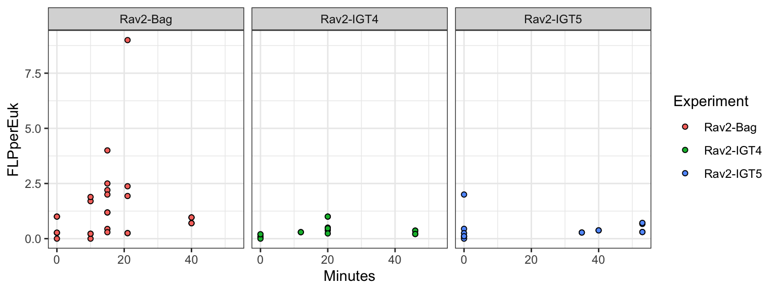

4.2 Calculate linear regression to obtain slope

Use lm() function in R to calculate linear regression for each experiment. Slope equates to grazing rate. Function inputs the FLP per euk cell data, performs regression and then adds a column for slope and r-squared values.

Function to estimate slope. Uses broom and tidymodels, then extracts slope.

Code

calculate_lm <- function(df){
  regression_1 <- df %>%
  type.convert(as.is = TRUE) %>%
  ## Keep technical replicates separate for IGTs
  group_by(SAMPLE, Site, Experiment, Name, IGT_REP, SizeFrac) %>%
  nest(-SAMPLE, -Site, -Experiment, -Name, -IGT_REP, -SizeFrac) %>%
  ## Combine technical replicates for IGTs
  # group_by(SAMPLE, Site, Experiment, Name, REP, SizeFrac) %>%
  # nest(-SAMPLE, -Site, -Experiment, -Name, -REP, -SizeFrac) %>%
  mutate(lm_fit = map(data, ~lm(FLPperEuk ~ Minutes, data = .)),
         tidied = map(lm_fit, tidy)) %>% 
  unnest(tidied) %>% 
  select(SAMPLE, Site, Experiment, Name, IGT_REP, SizeFrac, term, estimate) %>%
  # select(SAMPLE, Site, Experiment, Name, REP, SizeFrac, term, estimate) %>% 
  pivot_wider(names_from = term, values_from = estimate) %>% 
  data.frame
  # Reset column names
  colnames(regression_1) <- c("SAMPLE", "Site", 
                              "Experiment", "Name", "IGT_REP",
                              "SizeFrac", "INTERCEPT", "SLOPE")
  # Repeat broom model to get R2
  out_regression <- df %>%
  ## Keep technical replicates separate for IGTs
  group_by(SAMPLE, Site, Experiment, Name, IGT_REP, SizeFrac) %>%
  nest(-SAMPLE, -Site, -Experiment, -Name, -IGT_REP, -SizeFrac) %>%
  # group_by(SAMPLE, Site, Experiment, Name, REP, SizeFrac) %>%
  # nest(-SAMPLE, -Site, -Experiment, -Name, -REP, -SizeFrac) %>%
  mutate(lm_fit = map(data, ~lm(FLPperEuk ~ Minutes, data = .)),
         glanced = map(lm_fit, glance)) %>% 
  unnest(glanced) %>% 
    select(SAMPLE, Site, Experiment, Name, IGT_REP, SizeFrac, r.squared) %>%
    # select(SAMPLE, Site, Experiment, Name, REP, SizeFrac, r.squared) %>% 
  right_join(regression_1) %>% 
  right_join(df) %>% 
  data.frame
  out_regression$SITE <- factor(out_regression$Site, levels = c("VD", "Piccard"))
  out_regression$TYPE <- factor(out_regression$EXP_TYPE, levels = c("Bag", "IGT"))
  return(out_regression)
}

Note that an error may occur when running the below function. This is due to the fact that some experiments did not have replicates.

Apply to all data to obtain slope.

Code

calcs_wslope_regression <- calculate_lm(counts_flp_calcs_all)

Warning: Supplying `...` without names was deprecated in tidyr 1.0.0.
ℹ Please specify a name for each selection.
ℹ Did you want `data = c(-SAMPLE, -Site, -Experiment, -Name, -IGT_REP,
  -SizeFrac)`?

Warning: Supplying `...` without names was deprecated in tidyr 1.0.0.
ℹ Please specify a name for each selection.
ℹ Did you want `data = c(-SAMPLE, -Site, -Experiment, -Name, -IGT_REP,
  -SizeFrac)`?

Joining with `by = join_by(SAMPLE, Site, Experiment, Name, IGT_REP, SizeFrac)`
Joining with `by = join_by(SAMPLE, Site, Experiment, Name, IGT_REP, SizeFrac)`

gut check linear regression work. Use below commands out to recalculate one linear regression. Above function uses the nest() capability of tidyverse. Below, one experiment is subset to check the value.

Code

# Extract only plume-bag experiment from VD
# tmp_plume <- filter(counts_flp_calcs_all, Experiment == "Plume-Bag") %>% filter(Site == "VD") %>% filter(SizeFrac == "total_euks")
# # tmp_plume # View
# # Perform linear regression
# lm_out <- lm(FLPperEuk ~ Minutes, data = tmp_plume)
# # # Check output
# summary(lm_out)
# lm_out$coefficients #Intercept=intercept #Minutes = SLOPE
# # # Compare with nested function output
# filter(calcs_wslope_regression, Experiment == "Plume-Bag") %>% filter(Site == "VD") %>% filter(SizeFrac == "total_euks") %>% head

Plot linear regression trend

Plot all shipboard experiments with estimated slope.

Code

# | fig-width: 7
# | fig-height: 8
shipboardregression <- calcs_wslope_regression %>% 
  mutate(EXP_CATEGORY = case_when(
    EXP_TYPE == "Bag" ~ "Shipboard",
    TRUE ~ "IGT"
  )) %>% 
  mutate(EXP_CATEGORY_WREP = case_when(
    EXP_TYPE == "Bag" ~ "Shipboard",
    TRUE ~ IGT_REP
  )) %>% 
  # Factor name order and label
  mutate(SiteOrder = factor(Site, levels = site_ids, labels = site_fullname)) %>% 
  mutate(NameOrder = factor(Name, levels = vent_ids, labels = vent_fullname)) %>% 
  filter(SizeFrac == "total_euks") %>%
  ## Filter out IGT samples for now
  filter(TYPE != "IGT") %>%
  unite(EXPERIMENT, NameOrder, EXP_CATEGORY, sep = " ", remove = FALSE) %>% 
    ggplot(aes(x = Minutes, y = FLPperEuk, 
               fill = SiteOrder, color = SiteOrder, shape = EXP_CATEGORY)) +
    geom_abline(aes(slope = SLOPE, intercept = INTERCEPT), color = "black", linetype = "dashed", linewidth = 1) +
    geom_point(stat = "identity", 
               size = 2, aes(shape = EXP_CATEGORY, 
                             fill = SiteOrder, color = SiteOrder)) +
    scale_shape_manual(values = c(21, 21)) +
    scale_fill_manual(values = c("#E76F51", "#264653")) +
    scale_color_manual(values = c("#E76F51", "#264653")) +
  # scale_shape_manual(values = c(21, 21, 21, 21)) +
  #   scale_fill_manual(values = c("white", "#264653", "white", "#E76F51")) +
  #   scale_color_manual(values = c("#264653", "#264653", "#E76F51", "#E76F51")) +
    labs(x = "Minutes", y = bquote("FLP"~eukaryote^-1), title = "") +
    facet_wrap(SiteOrder ~ EXPERIMENT) +
    # Report r.squared
    geom_text(aes(x = 42, y = max(FLPperEuk), label = paste(round(SLOPE, 4))), 
              vjust = 1, hjust = 0, size = 3, color = "black") +
    theme_bw() + 
    theme(strip.background = element_blank(),
          strip.text = element_text(color = "black", size = 7),
                       legend.title = element_blank(),
                       legend.position = "right")
shipboardregression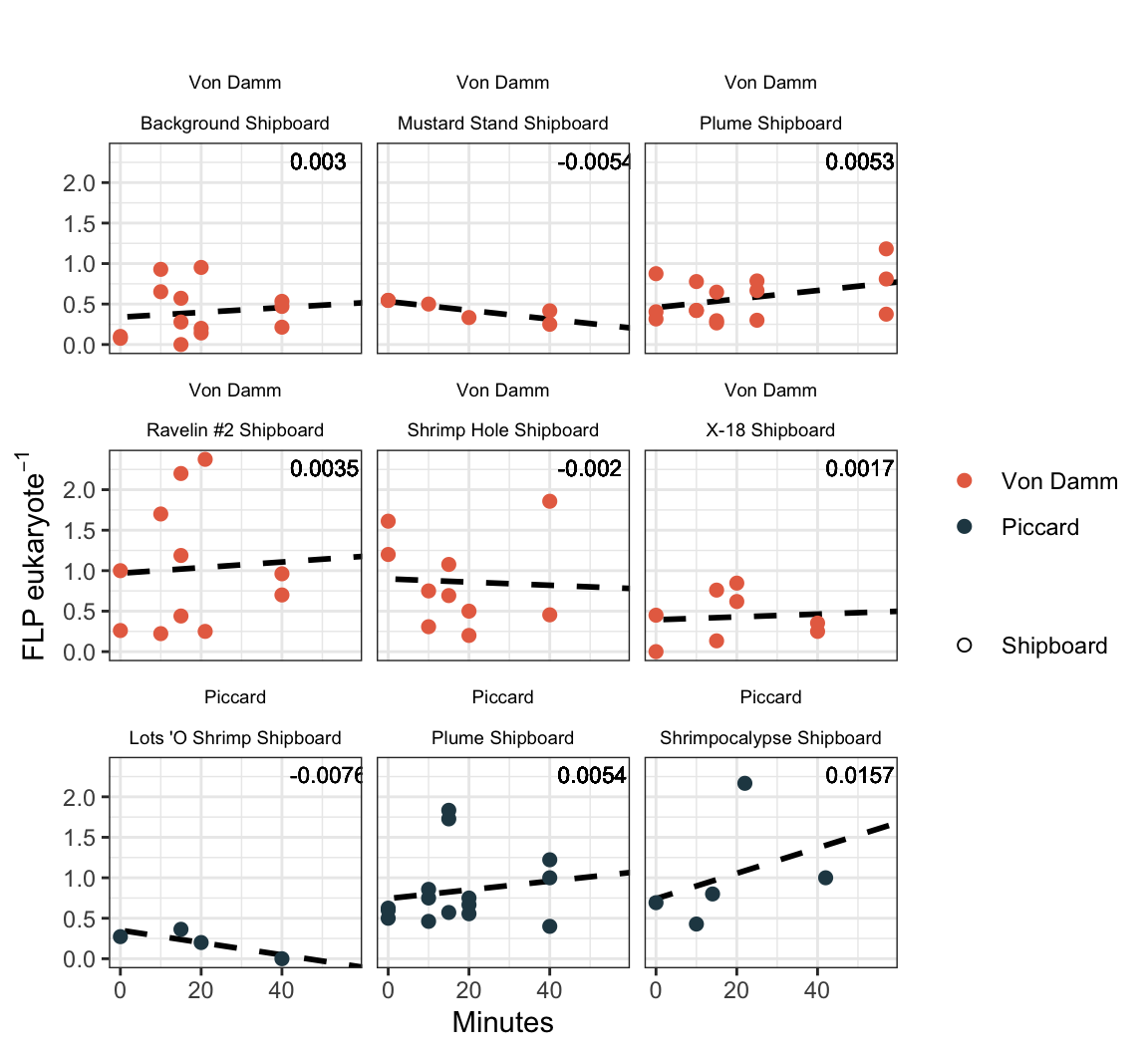

Data points represent the FLP per euk cells (based on total eukaryote cells counts). Y-axis represents the duration of incubation (in minutes). The dashed purple line reprents the slope and intercept of the experiment.

4.3 Remove IGT Tf time points.

IGT experiment results appear to have bottle effect, especially in the final time point. Additionally, due to the lack of biological replicates in the IGT experiments, technical replicates are treated as biological replicates in the regression below.

Code

IGT_lm_woTf <- counts_flp_calcs_all %>% 
  # Select only IGT experiments with total eukaryotes, remove Tf (T3)
  filter(SizeFrac == "total_euks") %>% 
  filter(EXP_TYPE == "IGT" & !(TimePoint == "T3")) %>% 
  # Remove repeated counts. Use this in supplement
  filter(!grepl("b", Replicate_ID)) %>% 
  add_column(IGT_cor = "rm Tf") %>% 
  data.frame

# Recalculate lm(), keep replicates separate
igt_regression_noTf <- calculate_lm(IGT_lm_woTf) # Recalculate

Warning: Supplying `...` without names was deprecated in tidyr 1.0.0.
ℹ Please specify a name for each selection.
ℹ Did you want `data = c(-SAMPLE, -Site, -Experiment, -Name, -IGT_REP,
  -SizeFrac)`?

Warning: Supplying `...` without names was deprecated in tidyr 1.0.0.
ℹ Please specify a name for each selection.
ℹ Did you want `data = c(-SAMPLE, -Site, -Experiment, -Name, -IGT_REP,
  -SizeFrac)`?

Joining with `by = join_by(SAMPLE, Site, Experiment, Name, IGT_REP, SizeFrac)`
Joining with `by = join_by(SAMPLE, Site, Experiment, Name, IGT_REP, SizeFrac)`

Plot IGT grazing experiments with newly calculated grazing effect.

Code

igtregression <- igt_regression_noTf %>% 
  # filter(SizeFrac == "total_euks") %>% 
  # filter(TYPE != "IGT") %>% 
  mutate(SITE_ORDER = factor(SITE, levels = site_ids, labels = site_fullname)) %>%
  unite(EXPERIMENT, SITE, Experiment, sep = " ", remove = FALSE) %>% 
  ggplot(aes(x = Minutes, y = FLPperEuk, fill = SITE_ORDER, shape = TYPE, group = Experiment)) +
  geom_abline(aes(slope = SLOPE, intercept = INTERCEPT), color = "black", linetype = "dashed", size = 1) +
  geom_point(stat = "identity", fill = "white", 
             size = 3, stroke = 2, aes(shape = TYPE, color = SITE_ORDER)) +
  scale_shape_manual(values = c(21, 21)) +
  scale_color_manual(values = site_color) +
  labs(x = "Minutes", y = bquote("FLP"~eukaryote^-1), title = "") +
  facet_wrap(. ~ EXPERIMENT) +
  # Report r.squared
  geom_text(aes(x = 5, y = max(FLPperEuk), label = paste(round(SLOPE, 4))), 
            vjust = 1, hjust = 0, size = 3) +
  theme_bw() + 
  theme(strip.background = element_blank(),
        strip.text = element_text(color = "black", size = 7),
                     legend.title = element_blank(),
                     legend.position = "right")

Warning: Using `size` aesthetic for lines was deprecated in ggplot2 3.4.0.
ℹ Please use `linewidth` instead.

Code

igtregression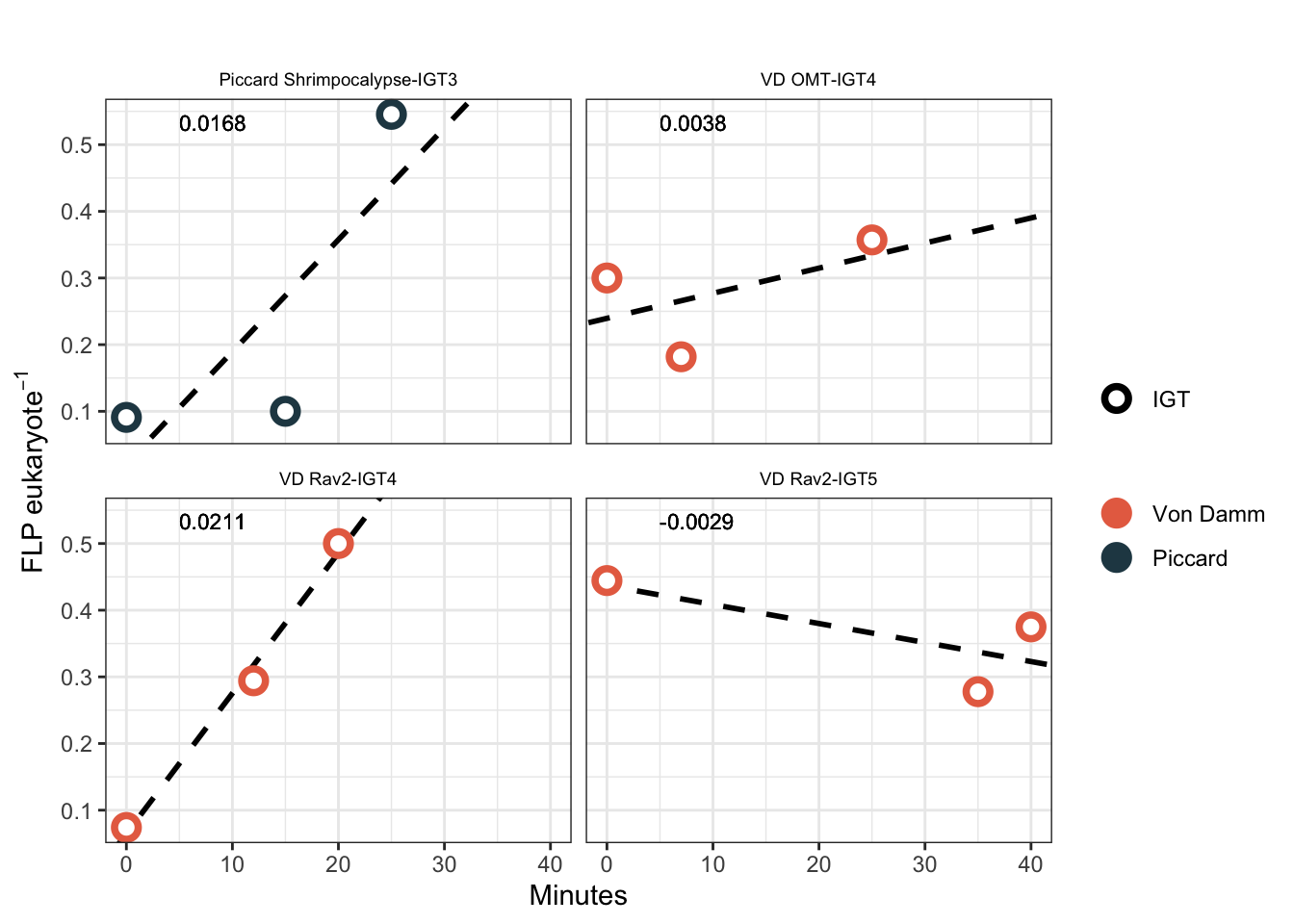

Results are more consistent across experiments when we remove Tf from the IGT experiments

Figure S4

Code

# svg("../../../Manuscripts_presentations_reviews/MCR-grazing-2023/svg-files-figures/figS3.svg", h = 12, w = 7)
shipboardregression + igtregression +
  patchwork::plot_layout(ncol = 1, heights = c(1, 0.7)) + patchwork::plot_annotation(tag_levels = "a")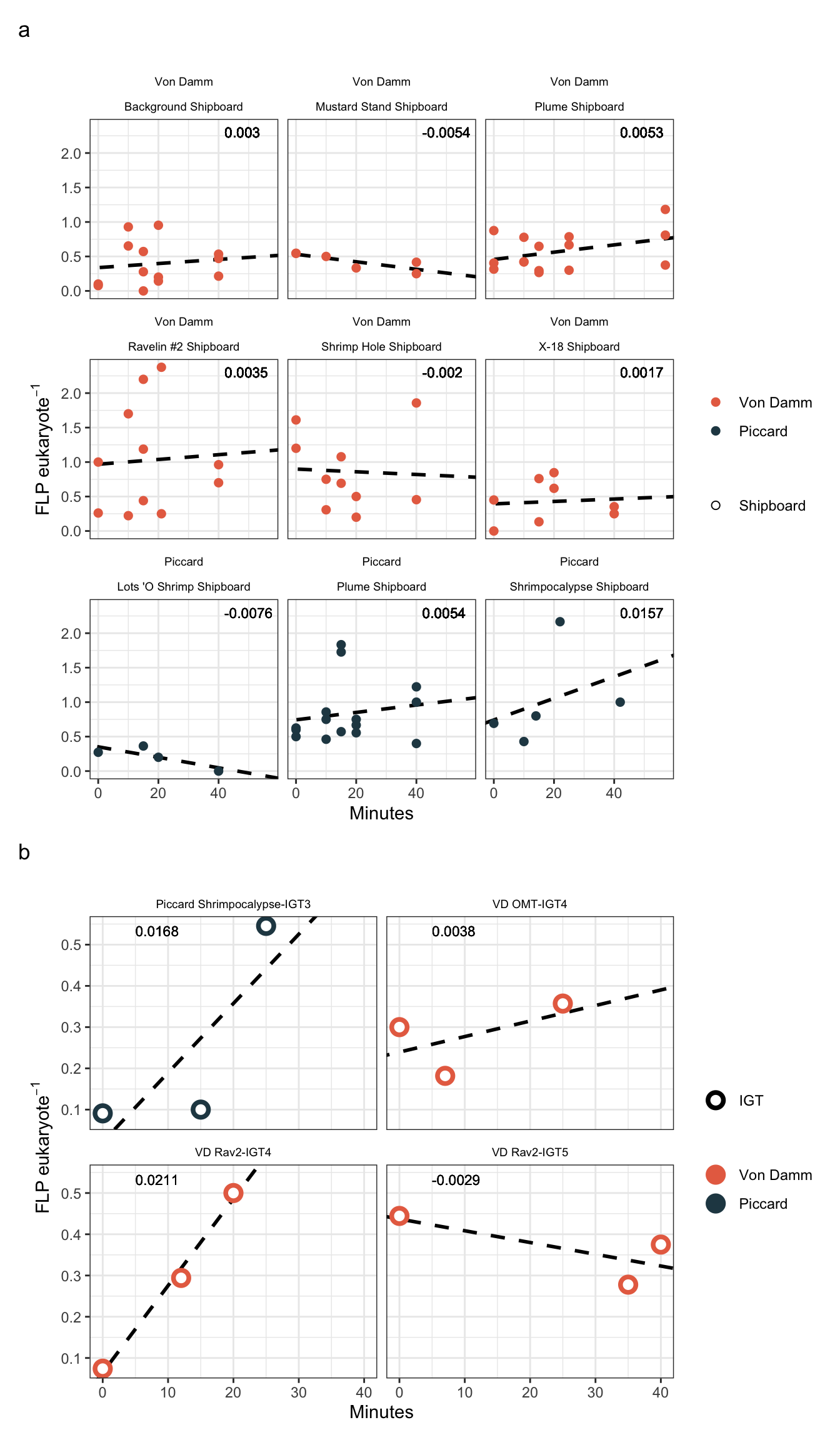

Code

# dev.off()

Repeat, but include technical replicates

Assess technical replicates for supplemental.

Code

IGT_lm_woTf_wb <- counts_flp_calcs_all %>% 
  # Select only IGT experiments with total eukaryotes, remove Tf (T3)
  filter(SizeFrac == "total_euks") %>% 
  filter(EXP_TYPE == "IGT" & !(TimePoint == "T3")) %>% 
  # Remove repeated counts. Use this in supplement
  # filter(!grepl("b", Replicate_ID)) %>% 
  add_column(IGT_cor = "rm Tf") %>% 
  # mutate(EXP_TYPE = IGT_REP) %>% 
  mutate(IGT_REP = Replicate_ID) %>% 
  unite("Experiment", Name, Replicate_ID, sep = "-", remove = FALSE) %>% 
  select(-REP, everything()) %>% 
  data.frame

# Recalculate lm(), keep replicates separate
igt_regression_noTf_wb <- calculate_lm(IGT_lm_woTf_wb) # Recalculate

Warning: Supplying `...` without names was deprecated in tidyr 1.0.0.
ℹ Please specify a name for each selection.
ℹ Did you want `data = c(-SAMPLE, -Site, -Experiment, -Name, -IGT_REP,
  -SizeFrac)`?

Warning: Supplying `...` without names was deprecated in tidyr 1.0.0.
ℹ Please specify a name for each selection.
ℹ Did you want `data = c(-SAMPLE, -Site, -Experiment, -Name, -IGT_REP,
  -SizeFrac)`?

Joining with `by = join_by(SAMPLE, Site, Experiment, Name, IGT_REP, SizeFrac)`
Joining with `by = join_by(SAMPLE, Site, Experiment, Name, IGT_REP, SizeFrac)`

Plot IGT grazing experiments with newly calculated slope.

Figure S9

Code

# svg("../../../Manuscripts_presentations_reviews/MCR-grazing-2023/svg-files-figures/figS9_new.svg")
igt_regression_noTf_wb %>% 
  # filter(SizeFrac == "total_euks") %>% 
  # filter(TYPE != "IGT") %>% 
  # Only isolate IGT 4s, where the technical replicates were done
  filter(grepl("IGT4", IGT_REP)) %>% 
  mutate(SITE_ORDER = factor(SITE, levels = site_ids, labels = site_fullname)) %>%
  unite(EXPERIMENT, SITE, Name, IGT_REP, sep = " ", remove = FALSE) %>% 
  ggplot(aes(x = Minutes, y = FLPperEuk, fill = SITE_ORDER, shape = TYPE, group = Experiment)) +
  geom_abline(aes(slope = SLOPE, intercept = INTERCEPT), color = "black", linetype = "dashed", size = 1) +
  geom_point(stat = "identity", fill = "white", 
             size = 3, stroke = 2, aes(shape = TYPE, color = SITE_ORDER)) +
  scale_shape_manual(values = c(21, 21)) +
  scale_color_manual(values = site_color) +
  labs(x = "Minutes", y = bquote("FLP"~eukaryote^-1), title = "Grazing experiment regression") +
  facet_wrap(. ~ EXPERIMENT) +
  # Report r.squared
  geom_text(aes(x = 5, y = max(FLPperEuk), label = paste(round(SLOPE, 4))), 
            vjust = 1, hjust = 0, size = 3) +
  theme_bw() + 
  theme(strip.background = element_blank(),
        strip.text = element_text(color = "black", size = 7),
                     legend.title = element_blank(),
                     legend.position = "right")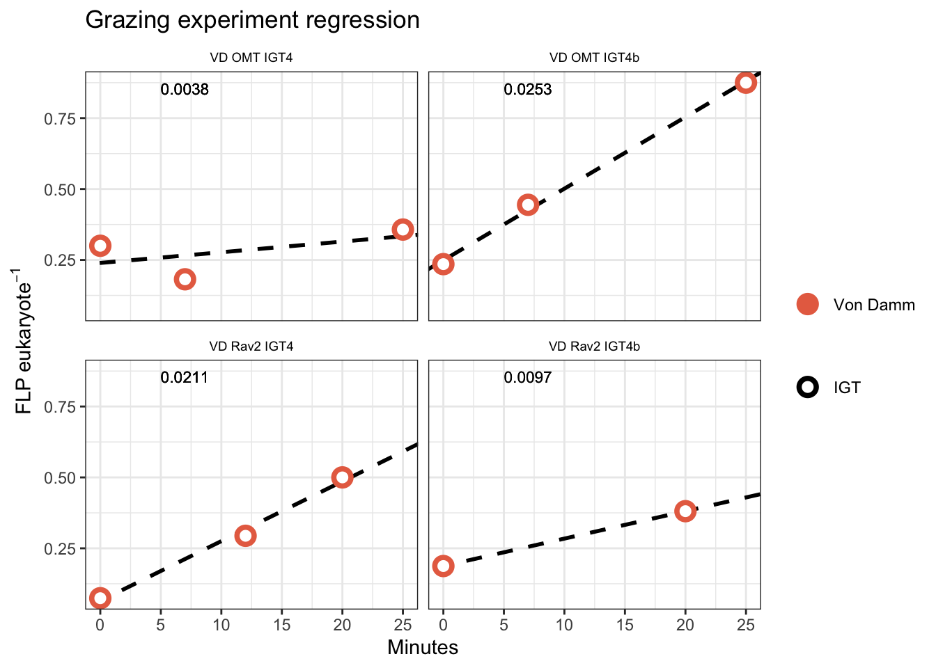

Code

# dev.off()

4.4 Compile and save grazing experiment results

Code

calcs_wslope_regression_update <- calcs_wslope_regression %>% 
  filter(TYPE != "IGT") %>% 
  bind_rows(igt_regression_noTf %>% select(-IGT_cor)) %>% 
  data.frame

# Factor
vent_ids <- c("BSW","Plume", "LotsOShrimp", "Shrimpocalypse", 
              "ShrimpHole", "X18", "Rav2", "MustardStand", "OMT")
vent_fullname <- c("Background","Plume", "Lots 'O Shrimp", "Shrimpocalypse",  
                   "Shrimp Hole", "X-18", "Ravelin #2", "Mustard Stand", "Old Man Tree")
site_ids <- c("VD", "Piccard")
site_fullname <- c("Von Damm", "Piccard")
# Factor for shipboard
calcs_wslope_regression_update$SiteOrder <- factor(calcs_wslope_regression_update$Site, levels = site_ids, labels = site_fullname)
calcs_wslope_regression_update$NameOrder <- factor(calcs_wslope_regression_update$Name, levels = vent_ids, labels = vent_fullname)

# View(calcs_wslope_regression_update)
calcs_wslope_regression_update %>%
  select(SiteOrigin, SiteOrder, NameOrder, Experiment, SizeFrac, r.squared, INTERCEPT, SLOPE) %>% distinct()

   SiteOrigin SiteOrder      NameOrder          Experiment   SizeFrac
1        Vent   Piccard Lots 'O Shrimp     LotsOShrimp-Bag total_euks
2       Plume   Piccard          Plume           Plume-Bag total_euks
3        Vent   Piccard Shrimpocalypse  Shrimpocalypse-Bag total_euks
4  Background  Von Damm     Background             BSW-Bag total_euks
5        Vent  Von Damm  Mustard Stand    MustardStand-Bag total_euks
6       Plume  Von Damm          Plume           Plume-Bag total_euks
7        Vent  Von Damm     Ravelin #2            Rav2-Bag total_euks
8        Vent  Von Damm    Shrimp Hole      ShrimpHole-Bag total_euks
9        Vent  Von Damm           X-18             X18-Bag total_euks
10       Vent   Piccard Lots 'O Shrimp     LotsOShrimp-Bag micro_size
11       Vent   Piccard Lots 'O Shrimp     LotsOShrimp-Bag  nano_size
12      Plume   Piccard          Plume           Plume-Bag micro_size
13      Plume   Piccard          Plume           Plume-Bag  nano_size
14       Vent   Piccard Shrimpocalypse  Shrimpocalypse-Bag micro_size
15       Vent   Piccard Shrimpocalypse  Shrimpocalypse-Bag  nano_size
16 Background  Von Damm     Background             BSW-Bag micro_size
17 Background  Von Damm     Background             BSW-Bag  nano_size
18       Vent  Von Damm  Mustard Stand    MustardStand-Bag micro_size
19       Vent  Von Damm  Mustard Stand    MustardStand-Bag  nano_size
20      Plume  Von Damm          Plume           Plume-Bag micro_size
21      Plume  Von Damm          Plume           Plume-Bag  nano_size
22       Vent  Von Damm     Ravelin #2            Rav2-Bag micro_size
23       Vent  Von Damm     Ravelin #2            Rav2-Bag  nano_size
24       Vent  Von Damm    Shrimp Hole      ShrimpHole-Bag micro_size
25       Vent  Von Damm    Shrimp Hole      ShrimpHole-Bag  nano_size
26       Vent  Von Damm           X-18             X18-Bag micro_size
27       Vent  Von Damm           X-18             X18-Bag  nano_size
28       Vent   Piccard Shrimpocalypse Shrimpocalypse-IGT3 total_euks
29       Vent  Von Damm   Old Man Tree            OMT-IGT4 total_euks
30       Vent  Von Damm     Ravelin #2           Rav2-IGT4 total_euks
31       Vent  Von Damm     Ravelin #2           Rav2-IGT5 total_euks
     r.squared   INTERCEPT        SLOPE
1  0.660252577  0.35170021 -0.007605829
2  0.028109981  0.74350881  0.005362856
3  0.134500775  0.74142021  0.015686872
4  0.016339803  0.33810711  0.002958889
5  0.679501856  0.53165317 -0.005445545
6  0.152459998  0.45659816  0.005274231
7  0.003588551  0.96801815  0.003470217
8  0.002436342  0.89841555 -0.001967253
9  0.007917377  0.39372646  0.001744429
10 0.000000000  0.50000000           NA
11 0.723950257  0.34152209 -0.007467037
12 0.031027392  1.84477124 -0.021241830
13 0.134388231  0.56572102  0.009146535
14 0.016488447  1.89710611 -0.016881029
15 0.219942841  0.57936763  0.022967165
16 0.289513467  1.45183824 -0.027181373
17 0.015152403  0.29347056  0.002856863
18 0.000000000  0.00000000           NA
19 0.679997859  0.52917792 -0.004985856
20 0.098467998  0.78410898  0.019766939
21 0.019373495  0.45137023  0.002263909
22 0.696359782 -1.71474878  0.394651540
23 0.001444937  0.93924980  0.002011385
24 0.233424455  2.28754579 -0.092124542
25 0.002819273  0.93709575  0.002424242
26 0.302757291  0.67091295  0.036093418
27 0.018916716  0.30417816  0.002196051
28 0.661389551  0.02153110  0.016794258
29 0.294853437  0.23949718  0.003764672
30 0.990856592  0.06472882  0.021062665
31 0.550820859  0.43701267 -0.002850877

Code

# write.csv(calcs_wslope_regression_update, file = "output-data/estimated-slopes-grazingexp.csv")

5 Check FLP control experiments

All incubations had control experiments run alongside them. This was to ensure added FLP did not decrease or change in concentration over time.

Code

bac_ctrl <- read.delim("input-data/bac-counts-compiled.txt")
# dim(bac_ctrl)
dtaf <- bac_ctrl %>% 
  mutate(ORIG_ID = Site) %>% 
  separate(SampleID, c("exp", "Replicate", "TimePoint"), sep = "-", remove = FALSE) %>% 
  separate(Site, c("Site", "Name"), sep = "-", remove = FALSE) %>% 
  filter(Stain == "DTAF") %>% 
  filter(!(Name == "Rav2" & Cells.ml > 90000)) %>% # remove inconsistent replicate from Ravelin #2
  filter(!(Name == "Rav2" & Replicate == "REP1")) %>% # remove inconsistent replicate from Ravelin #2
  data.frame

Warning: Expected 2 pieces. Additional pieces discarded in 17 rows [33, 34, 35, 36, 37,
38, 39, 40, 41, 42, 43, 44, 45, 46, 47, 48, 49].

Code

# 
dtaf_avg <- dtaf %>%
  group_by(TimePoint, Stain, Site, Name) %>%
  summarise(Avg_cellsperml = mean(Cells.ml),
            MIN = min(Cells.ml),
            MAX = max(Cells.ml)) %>%
  data.frame

`summarise()` has grouped output by 'TimePoint', 'Stain', 'Site'. You can
override using the `.groups` argument.

Code

# dtaf_avg

5.1 Bag grazing experiment controls

Option to plot averages. However, consistency between Replicate 1 and 2 was not always great. So plotting individually is best to show that the FLP do not disappear due to anomalous reasons.

Code

# bag_ctrls <- dtaf_avg %>% 
#   filter(Site != "IGT") %>% 
#   ggplot(aes(x = TimePoint, y = Avg_cellsperml, fill = Name, shape = Site)) +
#   geom_errorbar(aes(ymin = MIN, ymax = MAX), width = 0.1) +
#   geom_rect(data = filter(dtaf_avg, TimePoint == "T0", Site != "IGT"), aes(
#                                            ymin = (Avg_cellsperml-(0.15*Avg_cellsperml)),
#                                            ymax = (Avg_cellsperml+(0.15*Avg_cellsperml))), color = NA, alpha = 0.4, xmin = 0, xmax = 6, fill = "black") +
#   geom_line(aes(group = Name)) +
#   geom_point(stat = "identity", aes(shape = Site, fill = Name), size = 2) +
#   # scale_fill_manual(values = c("black","#9970ab", "#5aae61")) +
#   facet_wrap(Name ~ Site) +
#   scale_y_log10(labels = scientific_10) +
#   theme_bw() + theme(strip.background = element_blank(), 
#                           legend.title = element_blank(),
#                      axis.text = element_text(size = 10, color = "black"),
#                           title = element_text(size = 10, face = "bold"),
#                           axis.title = element_text(size = 9)) +
#   labs(title = "FLP counts for controls", y = bquote("Log FLP "~mL^-1), x = "Time point")
# bag_ctrls

Code

# View(dtaf)
ship_ctrls_reps <- dtaf %>% 
  filter(Site != "IGT") %>% 
  ggplot(aes(x = TimePoint, y = Cells.ml, fill = Name, shape = Replicate)) +
  geom_rect(data = filter(dtaf, TimePoint == "T0", Site != "IGT"), aes(
                                           ymin = (Cells.ml-(0.15*Cells.ml)),
                                           ymax = (Cells.ml+(0.15*Cells.ml))), color = NA, alpha = 0.4, xmin = 0, xmax = 6, fill = "black") +
  geom_line(aes(group = Replicate)) +
  geom_point(stat = "identity", aes(shape = Replicate), size = 2) +
  # scale_fill_manual(values = c("black","#9970ab", "#5aae61")) +
  facet_wrap(Name ~ Site) +
  scale_y_log10(labels = scientific_10) +
  theme_bw() + theme(strip.background = element_blank(), 
                          legend.title = element_blank(),
                     axis.text = element_text(size = 10, color = "black"),
                          title = element_text(size = 10, face = "bold"),
                          axis.title = element_text(size = 9)) +
  labs(title = "FLP counts for controls", y = bquote("Log FLP "~mL^-1), x = "Time point")
ship_ctrls_reps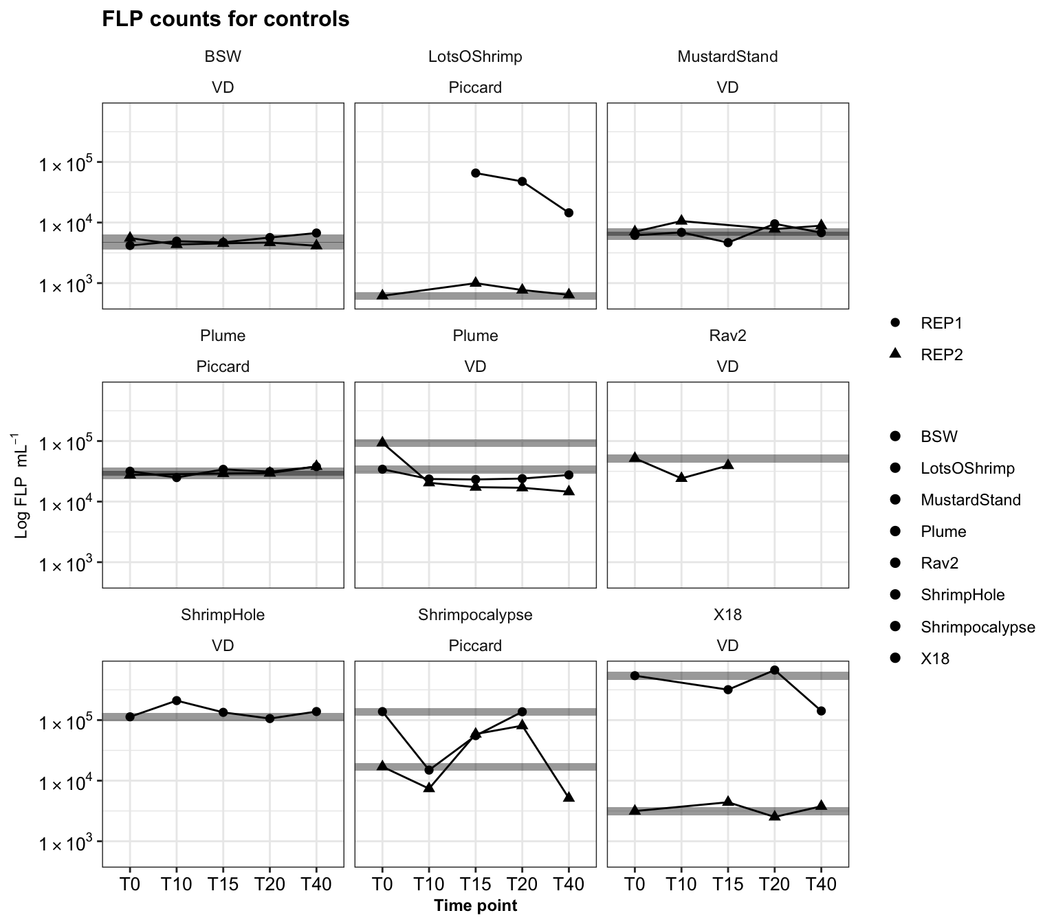

5.2 IGT experiment controls

Repeat for IGT experiments.

Code

igt_ctrl_reps <- dtaf %>% 
  filter(Site == "IGT") %>% 
  ggplot(aes(x = TimePoint, y = Cells.ml, shape = Replicate)) +
    geom_rect(data = filter(dtaf, TimePoint == "T0", Site == "IGT"), aes(
                                           ymin = (Cells.ml-(0.15*Cells.ml)),
                                           ymax = (Cells.ml+(0.15*Cells.ml))), color = NA, alpha = 0.4, xmin = 0, xmax = 6, fill = "black") +
  geom_line(aes(group = Replicate)) +
  geom_point(stat = "identity", aes(shape = Replicate), size = 2) +
  facet_wrap(Name ~ ORIG_ID) +
  scale_y_log10(labels = scientific_10) +
  theme_bw() + theme(strip.background = element_blank(), 
                          legend.title = element_blank(),
                     axis.text = element_text(size = 10, color = "black"),
                          title = element_text(size = 10, face = "bold"),
                          axis.title = element_text(size = 9)) +
  labs(title = "FLP counts for controls", y = bquote("Log FLP "~mL^-1), x = "Time point")
igt_ctrl_reps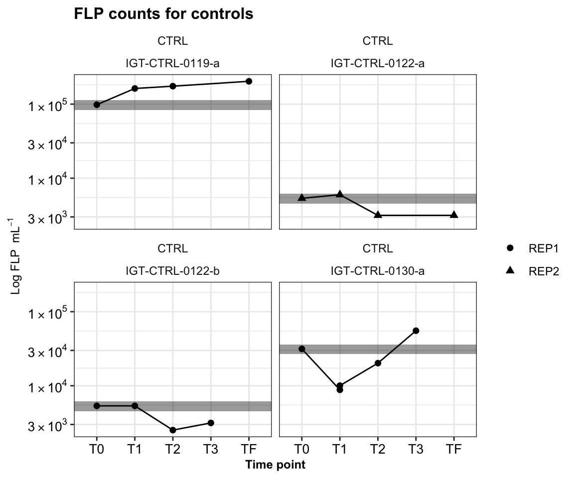

Figure S6

Code

# svg("../../../Manuscripts_presentations_reviews/MCR-grazing-2023/svg-files-figures/figS6_1.svg", w = 9, h = 7)
ship_ctrls_reps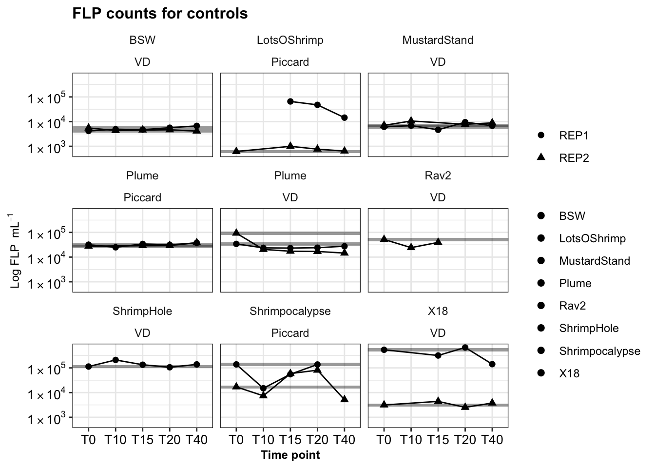

Code

# dev.off()

# svg("../../../Manuscripts_presentations_reviews/MCR-grazing-2023/svg-files-figures/figS6_2.svg", w = 7, h = 5)
igt_ctrl_reps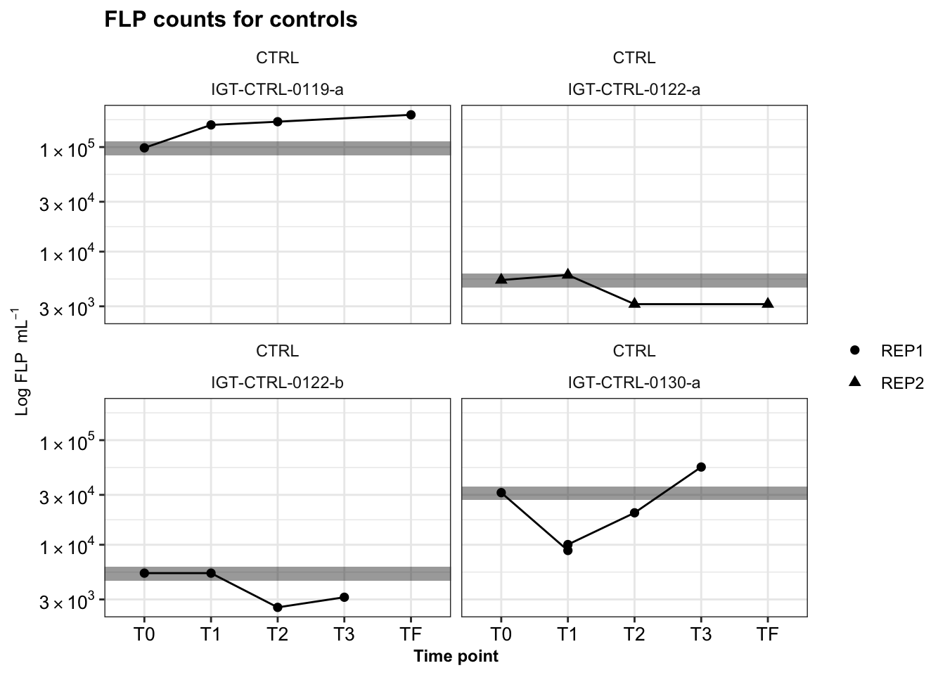

Code

# dev.off()

6 Generate complete table with grazing rates and values

Code

# head(calcs_wslope_regression_update)
# View(calcs_wslope_regression_update)
# Generate final table
bsw <- c("Plume", "Background")

table_grazerate <- calcs_wslope_regression_update %>% 
  filter(SizeFrac == "total_euks") %>% 
  select(SAMPLE, FLUID_ORIGIN, CRUISE_SAMPLE, SiteOrder, NameOrder, SLOPE, EXP_TYPE, EXP_REPS, EXP_VOL, CTRL_REPS, CTRL_VOL, IGT_REP, Site, Name, RATE = SLOPE, Minutes) %>% 
  distinct() %>% 
  group_by(SAMPLE, FLUID_ORIGIN, CRUISE_SAMPLE, IGT_REP, EXP_TYPE, EXP_REPS, EXP_VOL, CTRL_REPS, CTRL_VOL, Site, Name, SiteOrder, NameOrder, RATE) %>% 
  summarise(TimePoints = str_c(Minutes, collapse = ", ")) %>% 
  ungroup() %>%
  mutate(GRAZE_RATE = case_when(
    RATE < 0 ~ 0,
    TRUE ~ RATE
  ),
  type = case_when(
    Name == "Plume" ~ "Plume-Shipboard",
    Name == "Background" ~ "Background-Shipboard",
    EXP_TYPE == "IGT" ~ "Vent-IGT",
    EXP_TYPE == "Bag" ~ "Vent-Shipboard"
  ),
  LABEL_REPS = case_when(
    IGT_REP == "Bag" ~ "Shipboard",
    TRUE ~ IGT_REP
  )) %>%
  unite("Experiment_rep", Name, LABEL_REPS, sep = "-", remove = FALSE) %>% 
  data.frame

`summarise()` has grouped output by 'SAMPLE', 'FLUID_ORIGIN', 'CRUISE_SAMPLE',
'IGT_REP', 'EXP_TYPE', 'EXP_REPS', 'EXP_VOL', 'CTRL_REPS', 'CTRL_VOL', 'Site',
'Name', 'SiteOrder', 'NameOrder'. You can override using the `.groups`
argument.

Code

table_grazerate # view complete table of grazing rate results

                   SAMPLE FLUID_ORIGIN CRUISE_SAMPLE IGT_REP EXP_TYPE EXP_REPS
1     Piccard-LotsOShrimp      J2-1241          LV24     Bag      Bag        3
2           Piccard-Plume       CTD004     Niskin 10     Bag      Bag        3
3  Piccard-Shrimpocalypse      J2-1240          IGT3    IGT3      IGT        1
4  Piccard-Shrimpocalypse      J2-1240          LV13     Bag      Bag        3
5                  VD-BSW       CTD002  Niskins 8-10     Bag      Bag        3
6         VD-MustardStand      J2-1243          LV17     Bag      Bag        2
7                  VD-OMT      J2-1238          IGT4    IGT4      IGT        1
8                VD-Plume       CTD001      Niskin 2     Bag      Bag        3
9                 VD-Rav2      J2-1238         LV13a     Bag      Bag        3
10                VD-Rav2      J2-1244          IGT4    IGT4      IGT        1
11                VD-Rav2      J2-1244          IGT5    IGT5      IGT        1
12          VD-ShrimpHole      J2-1244          LV13     Bag      Bag        2
13                 VD-X18      J2-1235   LV23 & Bio5     Bag      Bag        2
   EXP_VOL CTRL_REPS CTRL_VOL    Site           Experiment_rep           Name
1     1.50         2      0.2 Piccard    LotsOShrimp-Shipboard    LotsOShrimp
2     2.00         2      0.5 Piccard          Plume-Shipboard          Plume
3     0.15        NA       NA Piccard      Shrimpocalypse-IGT3 Shrimpocalypse
4     1.50         2      0.2 Piccard Shrimpocalypse-Shipboard Shrimpocalypse
5     2.00         2      0.5      VD            BSW-Shipboard            BSW
6     1.50         2      0.2      VD   MustardStand-Shipboard   MustardStand
7     0.15        NA       NA      VD                 OMT-IGT4            OMT
8     2.00         2      1.0      VD          Plume-Shipboard          Plume
9     1.50         2      0.5      VD           Rav2-Shipboard           Rav2
10    0.15        NA       NA      VD                Rav2-IGT4           Rav2
11    0.15        NA       NA      VD                Rav2-IGT5           Rav2
12    1.50         2      0.2      VD     ShrimpHole-Shipboard     ShrimpHole
13    1.50         2      0.5      VD            X18-Shipboard            X18
   SiteOrder      NameOrder         RATE        TimePoints  GRAZE_RATE
1    Piccard Lots 'O Shrimp -0.007605829     0, 15, 20, 40 0.000000000
2    Piccard          Plume  0.005362856 0, 10, 15, 20, 40 0.005362856
3    Piccard Shrimpocalypse  0.016794258         0, 15, 25 0.016794258
4    Piccard Shrimpocalypse  0.015686872 0, 10, 14, 22, 42 0.015686872
5   Von Damm     Background  0.002958889 0, 10, 15, 20, 40 0.002958889
6   Von Damm  Mustard Stand -0.005445545     0, 10, 20, 40 0.000000000
7   Von Damm   Old Man Tree  0.003764672          0, 7, 25 0.003764672
8   Von Damm          Plume  0.005274231 0, 10, 15, 25, 57 0.005274231
9   Von Damm     Ravelin #2  0.003470217 0, 10, 15, 21, 40 0.003470217
10  Von Damm     Ravelin #2  0.021062665         0, 12, 20 0.021062665
11  Von Damm     Ravelin #2 -0.002850877         0, 35, 40 0.000000000
12  Von Damm    Shrimp Hole -0.001967253 0, 10, 15, 20, 40 0.000000000
13  Von Damm           X-18  0.001744429     0, 15, 20, 40 0.001744429
              type LABEL_REPS
1   Vent-Shipboard  Shipboard
2  Plume-Shipboard  Shipboard
3         Vent-IGT       IGT3
4   Vent-Shipboard  Shipboard
5   Vent-Shipboard  Shipboard
6   Vent-Shipboard  Shipboard
7         Vent-IGT       IGT4
8  Plume-Shipboard  Shipboard
9   Vent-Shipboard  Shipboard
10        Vent-IGT       IGT4
11        Vent-IGT       IGT5
12  Vent-Shipboard  Shipboard
13  Vent-Shipboard  Shipboard

Code

table_grazerate %>% 
  group_by(Experiment_rep, Site) %>% 
  summarise(mean_rate = mean(GRAZE_RATE),
            min_rate = min(GRAZE_RATE),
            max = max(GRAZE_RATE))

`summarise()` has grouped output by 'Experiment_rep'. You can override using
the `.groups` argument.

# A tibble: 13 × 5
# Groups:   Experiment_rep [12]
   Experiment_rep           Site    mean_rate min_rate     max
   <chr>                    <chr>       <dbl>    <dbl>   <dbl>
 1 BSW-Shipboard            VD        0.00296  0.00296 0.00296
 2 LotsOShrimp-Shipboard    Piccard   0        0       0      
 3 MustardStand-Shipboard   VD        0        0       0      
 4 OMT-IGT4                 VD        0.00376  0.00376 0.00376
 5 Plume-Shipboard          Piccard   0.00536  0.00536 0.00536
 6 Plume-Shipboard          VD        0.00527  0.00527 0.00527
 7 Rav2-IGT4                VD        0.0211   0.0211  0.0211 
 8 Rav2-IGT5                VD        0        0       0      
 9 Rav2-Shipboard           VD        0.00347  0.00347 0.00347
10 ShrimpHole-Shipboard     VD        0        0       0      
11 Shrimpocalypse-IGT3      Piccard   0.0168   0.0168  0.0168 
12 Shrimpocalypse-Shipboard Piccard   0.0157   0.0157  0.0157 
13 X18-Shipboard            VD        0.00174  0.00174 0.00174

Code

table_grazerate %>% 
  mutate(TYPE = case_when(
    Name == "Plume" ~ "non-vent",
    Name == "Background" ~ "non-vent",
    TRUE ~ "vent"
  )) %>% 
  # group_by(Site, TYPE) %>% 
  # group_by(TYPE) %>%
  group_by(TYPE, EXP_TYPE) %>% 
  summarise(mean_rate = mean(GRAZE_RATE),
            min_rate = min(GRAZE_RATE),
            max = max(GRAZE_RATE))

`summarise()` has grouped output by 'TYPE'. You can override using the
`.groups` argument.

# A tibble: 3 × 5
# Groups:   TYPE [2]
  TYPE     EXP_TYPE mean_rate min_rate     max
  <chr>    <chr>        <dbl>    <dbl>   <dbl>
1 non-vent Bag        0.00532  0.00527 0.00536
2 vent     Bag        0.00341  0       0.0157 
3 vent     IGT        0.0104   0       0.0211 

Amend table with estimated FLP concentration

Code

# head(table_grazerate)
dtaf_igt <- 5352.8278 # Manually insert FLP concentration for IGT experiments; this value is estimated from how IGT FLP spike-ins were calculated
# 
table_grazerate_wflp <- bac_ctrl %>%
  filter(FLP_t0 == "use") %>%
  add_column(EXP_TYPE = "Bag") %>%
  group_by(Site, EXP_TYPE) %>%
  summarise(FLP_conc = mean(Cells.ml)) %>% 
  right_join(table_grazerate, by = c("Site" = "SAMPLE", "EXP_TYPE" = "EXP_TYPE")) %>%
  mutate(FLP_ml = ifelse(EXP_TYPE == "IGT", dtaf_igt, FLP_conc)) %>%
  select(everything(), FIELD = `Site.y`, -FLP_conc) %>% 
  data.frame

`summarise()` has grouped output by 'Site'. You can override using the
`.groups` argument.

Introduce factors in table for visualizations

Code

type_order <- c("Vent-Bag", "Vent-IGT", "Plume", "Background")
table_grazerate_wflp$TYPE <- factor(table_grazerate_wflp$type, levels = type_order)
vent_ids <- c("BSW","Plume", "LotsOShrimp", "Shrimpocalypse", 
              "ShrimpHole", "X18", "Rav2", "MustardStand", "OMT")
vent_fullname <- c("Background","Plume", "Lots 'O Shrimp", "Shrimpocalypse",  
                   "Shrimp Hole", "X-18", "Ravelin #2", "Mustard Stand", "Old Man Tree")
site_ids <- c("VD", "Piccard")
site_fullname <- c("Von Damm", "Piccard")
site_color <- c("#E76F51", "#264653")
names(site_color) <- site_fullname
table_grazerate_wflp$FIELDORDER <- factor(table_grazerate_wflp$FIELD, levels = site_ids, labels = site_fullname)
table_grazerate_wflp$VENTORDER <- factor(table_grazerate_wflp$Name, levels = vent_ids, labels = vent_fullname)

# table_grazerate_wflp

6.1 Plot FLP/grazer /minute

Code

# svg("", h =, w = )
grazing_min_plot <- table_grazerate_wflp %>% 
  mutate(EXP_CATEGORY = case_when(
    EXP_TYPE == "Bag" ~ "Shipboard",
    TRUE ~ "IGT"
  )) %>% 
  mutate(EXP_CATEGORY_WREP = case_when(
    EXP_TYPE == "Bag" ~ "Shipboard",
    TRUE ~ IGT_REP
  )) %>% 
  unite("SITE_TYPE", FIELD, EXP_CATEGORY, sep = "-", remove = FALSE) %>%
  ggplot(aes(y = GRAZE_RATE, x = VENTORDER, shape = SITE_TYPE, 
             fill = SITE_TYPE, color = SITE_TYPE)) +
  geom_jitter(stat = "identity", aes(shape = SITE_TYPE, 
                                     fill = SITE_TYPE, color = SITE_TYPE),
              stroke = 2, size = 3, width = 0.25) +
    scale_shape_manual(values = c(21, 21, 21, 21)) +
    scale_fill_manual(values = c("white", "#264653", "white", "#E76F51")) +
    scale_color_manual(values = c("#264653", "#264653", "#E76F51", "#E76F51")) +
  facet_grid(.~FIELDORDER, space = "free", scales = "free") +
  # coord_flip() +
    theme_minimal() +
    theme(panel.grid.major = element_line(), panel.grid.minor = element_blank(),
           panel.background = element_blank(), 
           axis.line = element_line(colour = "black"), 
           axis.text.x = element_text(color="black", size = 13, 
                                      angle = 45, hjust = 1, vjust = 1), 
           axis.text.y = element_text(color="black", size = 13),
           axis.title =element_text(color="black", size = 13),
           axis.ticks = element_line(),
           strip.text =element_blank(), legend.title = element_blank(),
          legend.position = "top") +
    labs(x = "", y = bquote("Average FLP " ~grazer^-1 ~min^-1))
# dev.off()
grazing_min_plot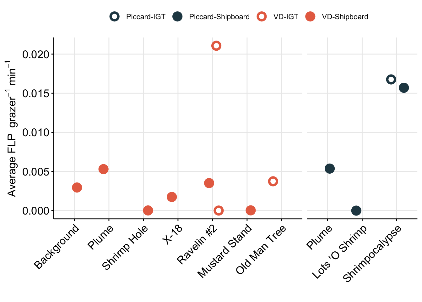

Table 1

Create table with all base experiment results. Including, grazing rate derived from slope (and corrected), number of experiments, replicates, and prok and euk counts.

For IGT experiments, or experiments where in situ prok counts were not obtained, the average in situ prok count was used.

Code

# Subset the average in situ prok cells/ml for non-background samples
tmp <- filter(insitu_proks, Name != "BSW", Name != "Plume") %>% select(MEAN)
avg_insitu <- mean(tmp$MEAN)

# View(table_grazerate_wflp)
# View(euk_prok_counts)

table_grazerate_wflp_wprok_weuk <- table_grazerate_wflp %>% 
  select(Experiment_rep, FIELD, Name, SiteOrder, NameOrder, FLUID_ORIGIN, CRUISE_SAMPLE, RATE, RATE_minute = GRAZE_RATE, FLP_ml, TimePoints, EXP_REPS, EXP_VOL, CTRL_REPS, CTRL_VOL) %>% 
  full_join(euk_prok_counts, join_by(Experiment_rep == Experiment_rep, Name == Name, FIELD == Site)) %>% 
  mutate(PROK_ml = ifelse(is.na(PROK_ml), avg_insitu, PROK_ml))

# table_grazerate_wflp_wprok_weuk
# names(table_grazerate_wflp_wprok_weuk)

Description of variables above:

• FIELD - vent location
• NAME - name of vent site, or plume/background
• EXP - experiment type, bag or IGT
• SAMPLE - vent site
• RATE_minute = GRAZE_RATE - FLPs per grazer per minute (SLOPE of best fitline)
• FLP_ml - FLP concentration at T0
• Prok_ml, sem - concentration and standard mean error of concentration of prokaryotes
• Euk_ml, sem - concentration and standard mean error of concentration of eukaryotes.

7 Grazing rate calculations

Based on Unrein et al. 2007, we use the estimated grazing rate, in situ prok abundance, in situ euk abundance, and the concentration of FLP to make additional estimates.

Code

# head(table_grazerate_wflp_wprok_weuk)
table_wcalcs <- table_grazerate_wflp_wprok_weuk %>%
  # Ingestion rate per hour
  mutate(RATE_hr = (RATE_minute * 60),
         RATE_day = (RATE_hr * 24), #Compare to GR?
         # FLP concentration per L
         FLP_L = (FLP_ml * 1000),
         # mL per grazer per hr
         CLEARANCE_RATE_ml = (RATE_hr/FLP_ml),
         # nL per grazer per hour
         CLEARANCE_RATE_nL = ((RATE_hr/FLP_ml)/1.00E+6), 
         # proks per grazer per hr
         SPEC_GRAZE_RATE_hr = (CLEARANCE_RATE_ml * PROK_ml), 
         # proks per grazer per day
         GRAZE_RATE_DAY = (24 * SPEC_GRAZE_RATE_hr),
         # proks per ml per hr
         GRAZING_EFFECT_hr = (SPEC_GRAZE_RATE_hr * EUK_ml),
         GRAZING_EFFECT_hr_min = (SPEC_GRAZE_RATE_hr * (EUK_ml - EUK_sem)),
         GRAZING_EFFECT_hr_max = (SPEC_GRAZE_RATE_hr * (EUK_ml + EUK_sem)),
         # cells per ml per day
         GRAZING_EFFECT_day = ((SPEC_GRAZE_RATE_hr * 24) * EUK_ml),
         # Percentage per day
         BAC_TURNOVER_PERC = 100*(GRAZING_EFFECT_day / PROK_ml),
         BAC_TURNOVER_PERC_min = 100*(GRAZING_EFFECT_day / (PROK_ml - PROK_sem)),
         BAC_TURNOVER_PERC_max = 100*(GRAZING_EFFECT_day / (PROK_ml + PROK_sem))) %>% 
  data.frame
# View(table_wcalcs)
# write_delim(table_wcalcs, file = "output-data/table-wcalc.txt", delim = "\t")

Explanation of units for table with calculated values.

• RATE_min & RATE_hr = Grazing rate as ‘FLPs per grazer per minute’ and per hour

• CLEARANCE_RATE = ml or nL per grazer per hour

• SPEC_GRAZE_RATE (Specific grazing rate) = Prokaryotes per grazer per hour

• GRAZING EFFECT = bacteria per ml per hour

• Bacterial turnover rate = % per day

Table 1 and S1 - grazing experiment information only

Code

# ## Table 1
# write_delim(table_wcalcs %>%
              # select(SiteOrder, NameOrder, FLUID_ORIGIN, CRUISE_SAMPLE, EUK_ml, EUK_MinMax, PROK_ml, PROK_MinMax, GRAZING_EFFECT_hr, RATE_minute, CLEARANCE_RATE_ml, BAC_TURNOVER_PERC),
#             file = "output-data/table1-grazing-exp-list.txt", delim = "\t")
# # 
# # ## Table S2
# write_delim(table_wcalcs %>%
#               select(SiteOrder, NameOrder, FLUID_ORIGIN, CRUISE_SAMPLE,
#                      TimePoints, starts_with("EXP"), starts_with("CTRL"), EUK_ml, EUK_MinMax, EUK_sem, PROK_ml, PROK_MinMax, PROK_sem, FLP_ml, GRAZE_RATE_DAY, Slope = RATE, RATE_minute, GRAZING_EFFECT_hr, CLEARANCE_RATE_ml, BAC_TURNOVER_PERC),
#             file = "output-data/tableS2-grazing-exp-list.txt", delim = "\t")

8 Carbon biomass for eukaryotes

References for estimating biovolume Pernice, M.C., Forn, I., Gomes, A., Lara, E., Alonso-Sáez, L., Arrieta, J.M., et al. (2015) Global abundance of planktonic heterotrophic protists in the deep ocean. ISME J 9: 782–792.

Code

# Import manual biovolume measurements
biov <- read.delim("input-data/biovol-euk-12-10-2020.txt")
# head(biov)

8.1 C factor based on biovolume

1. Calculate biovolume based on observed/imaged cells

Code

# Calculate biovolume, then apply carbon by biomass estimate for protists derived from biovolume.
# h = largest cell dimension "height"
# d = largest cross-section of h
biov_calc <- biov %>% 
  mutate(BIOVOLUME = ((pi/6) * (d^2) * h)) %>% # Calculate volume (um cubed) # Hillebrand et al. 1999
  mutate(pgC_cell_MD_dino = (0.760 * (BIOVOLUME^0.819))) %>% # Menden-Deuer and Lessard 2000
  mutate(pgC_cell_MD_nodiatom = (0.216 * (BIOVOLUME^0.939))) # Menden-Deuer and Lessard 2000
# head(biov_calc)
# biov_calc
# mean(c(80, 360))
# no diatom is what Pernice used.

Use pgC_cell_MD_nodiatom moving forward.

2. Get a summary pg per cell for vent and background samples. This is derived from biovolume estimates.

8.2 Biomass summaries

Code

c_factor_biov <- 
  biov_calc %>% select(-EXP, -h, -d) %>% 
  pivot_longer(cols = c(BIOVOLUME, starts_with("pgC_")), names_to = "VARIABLES", values_to = "VALUES") %>% 
  group_by(VENT_BSW, VARIABLES) %>% 
    summarise(mean = mean(VALUES),
              max = max(VALUES),
              min = min(VALUES)) %>% 
  pivot_wider(names_from = VENT_BSW, values_from = c(mean, max,min), names_sort = FALSE)

`summarise()` has grouped output by 'VENT_BSW'. You can override using the
`.groups` argument.

Code

# View(c_factor_biov)

3. Assign a C conversion factor for background and within vents based on biovolume

Code

# pg C per cell (pgC_cell)

pgC_cell_BSW <- subset(c_factor_biov, VARIABLES == "pgC_cell_MD_nodiatom")$mean_BSW

pgC_cell_vent <- subset(c_factor_biov, VARIABLES == "pgC_cell_MD_nodiatom")$mean_vent

pgC_cell_BSW_min <- subset(c_factor_biov, VARIABLES == "pgC_cell_MD_nodiatom")$min_BSW

pgC_cell_vent_min <- subset(c_factor_biov, VARIABLES == "pgC_cell_MD_nodiatom")$min_vent

pgC_cell_BSW_max <- subset(c_factor_biov, VARIABLES == "pgC_cell_MD_nodiatom")$max_BSW

pgC_cell_vent_max <- subset(c_factor_biov, VARIABLES == "pgC_cell_MD_nodiatom")$max_vent

pgC_cell_BSW

[1] 109.1574

Code

pgC_cell_vent

[1] 414.8068

4. Combine with count table to estimate total standing stock in carbon

Isolate at T0 all the euk cells per ml counts. Then add in the mean, min/max for the pg C per cell, based on the vent vs non-vent.

Code

# counts_cellsml_avg
pgC_ml_biov_bysample <- counts_cellsml_avg %>% 
  filter(TimePoint == "T0") %>%
  filter(VARIABLE == "eukCONC") %>% 
  mutate(SAMPLE_TYPE_BIN = case_when(
    Name == "Background" ~ "Non-vent",
    Name == "Plume" ~ "Non-vent",
    TRUE ~ "Vent"
  )) %>% 
  # pg C per ml = (cells per ml)*(pg C per)
  ## Apply the non-vent and vent pg C per cell value to total cells per ml
  mutate(pgC_ml_mean = case_when(
    SAMPLE_TYPE_BIN == "Non-vent" ~ MEAN * pgC_cell_BSW,
    SAMPLE_TYPE_BIN == "Vent" ~ MEAN * pgC_cell_vent,
  )) %>% 
  mutate(pgC_ml_min = case_when(
    SAMPLE_TYPE_BIN == "Non-vent" ~ MEAN * pgC_cell_BSW_min,
    SAMPLE_TYPE_BIN == "Vent" ~ MEAN * pgC_cell_vent_min
  )) %>% 
  mutate(pgC_ml_max = case_when(
    SAMPLE_TYPE_BIN == "Non-vent" ~ MEAN * pgC_cell_BSW_max,
    SAMPLE_TYPE_BIN == "Vent" ~ MEAN * pgC_cell_vent_max
  )) %>% 
  mutate(IGT_REP = case_when(
    IGT_REP == "Bag" ~ "Shipboard",
    TRUE ~ IGT_REP
  )) %>% 
  unite("Experiment_rep", Name, IGT_REP, sep = "-", remove = FALSE)

pgC_ml_biov_bysample

      Site           Experiment_rep           Name TimePoint EXP_TYPE   IGT_REP
1  Piccard    LotsOShrimp-Shipboard    LotsOShrimp        T0      Bag Shipboard
2  Piccard          Plume-Shipboard          Plume        T0      Bag Shipboard
3  Piccard Shrimpocalypse-Shipboard Shrimpocalypse        T0      Bag Shipboard
4  Piccard      Shrimpocalypse-IGT3 Shrimpocalypse        T0      IGT      IGT3
5  Piccard      Shrimpocalypse-IGT7 Shrimpocalypse        T0      IGT      IGT7
6       VD            BSW-Shipboard            BSW        T0      Bag Shipboard
7       VD   MustardStand-Shipboard   MustardStand        T0      Bag Shipboard
8       VD                 OMT-IGT4            OMT        T0      IGT      IGT4
9       VD                OMT-IGT4b            OMT        T0      IGT     IGT4b
10      VD          Plume-Shipboard          Plume        T0      Bag Shipboard
11      VD           Rav2-Shipboard           Rav2        T0      Bag Shipboard
12      VD                Rav2-IGT4           Rav2        T0      IGT      IGT4
13      VD               Rav2-IGT4b           Rav2        T0      IGT     IGT4b
14      VD                Rav2-IGT5           Rav2        T0      IGT      IGT5
15      VD               Rav2-IGT5b           Rav2        T0      IGT     IGT5b
16      VD     ShrimpHole-Shipboard     ShrimpHole        T0      Bag Shipboard
17      VD            X18-Shipboard            X18        T0      Bag Shipboard
   VARIABLE      MEAN        VAR        SD        SEM       MIN      MAX
1   eukCONC 230.90630         NA        NA         NA 230.90630 230.9063
2   eukCONC  79.30115   848.6444  29.13150  16.819081  55.97728 111.9546
3   eukCONC 454.81543         NA        NA         NA 454.81543 454.8154
4   eukCONC 384.84383         NA        NA         NA 384.84383 384.8438
5   eukCONC 524.78704         NA        NA         NA 524.78704 524.7870
6   eukCONC  91.83773   956.2550  30.92337  21.866127  69.97160 113.7039
7   eukCONC 259.76958  1666.1787  40.81885  28.863287 230.90630 288.6329
8   eukCONC 349.85802         NA        NA         NA 349.85802 349.8580
9   eukCONC 594.75864         NA        NA         NA 594.75864 594.7586
10  eukCONC 157.77468 13506.6620 116.21817  67.098589  55.97728 284.4007
11  eukCONC 409.33389 10795.7362 103.90253  73.470185 335.86370 482.8041
12  eukCONC 944.61667         NA        NA         NA 944.61667 944.6167
13  eukCONC 559.77284         NA        NA         NA 559.77284 559.7728
14  eukCONC 629.74444         NA        NA         NA 629.74444 629.7444
15  eukCONC 349.85802         NA        NA         NA 349.85802 349.8580
16  eukCONC 385.71847   123.9306  11.13241   7.871806 377.84667 393.5903
17  eukCONC 314.87222 22032.1147 148.43219 104.957407 209.91481 419.8296
   SAMPLE_TYPE_BIN pgC_ml_mean pgC_ml_min pgC_ml_max
1             Vent   95781.500  1216.6456  296465.66
2         Non-vent    8656.305  2241.3730   20432.20
3             Vent  188660.531  2396.4232  583947.52
4             Vent  159635.834  2027.7427  494109.44
5             Vent  217685.228  2765.1037  673785.60
6             Vent   38094.915   483.8932  117912.48
7             Vent  107754.188  1368.7263  333523.87
8             Vent  145123.485  1843.4025  449190.40
9             Vent  246709.925  3133.7842  763623.68
10        Non-vent   17222.270  4459.3540   40651.15
11            Vent  169794.478  2156.7809  525552.77
12            Vent  391833.410  4977.1867 1212814.08
13            Vent  232197.576  2949.4440  718704.64
14            Vent  261222.273  3318.1245  808542.72
15            Vent  145123.485  1843.4025  449190.40
16            Vent  159998.642  2032.3512  495232.42
17            Vent  130611.137  1659.0622  404271.36

Table reports the total pg of carbon per ml when we consider the whole eukaryote community (based on cell count).

Report in pg of C per ml.

Code

vent_ids <- c("BSW","Plume", "LotsOShrimp", "Shrimpocalypse", 
              "ShrimpHole", "X18", "Rav2", "MustardStand", "OMT")
vent_fullname <- c("Background","Plume", "Lots 'O Shrimp", "Shrimpocalypse",  
                   "Shrimp Hole", "X-18", "Ravelin #2", "Mustard Stand", "Old Man Tree")
site_ids <- c("VD", "Piccard")
site_fullname <- c("Von Damm", "Piccard")

by_biovol_plot <- pgC_ml_biov_bysample %>% 
  mutate(NameOrder = factor(Name, levels = vent_ids, labels = vent_fullname)) %>%
  mutate(SiteOrder = factor(Site, levels = site_ids, labels = site_fullname)) %>% 
  ggplot(aes(x = Experiment_rep, y = (pgC_ml_mean))) +
    geom_point(shape = 21, color = "black") + 
    geom_linerange(aes(ymin = (pgC_ml_min), ymax = (pgC_ml_max))) +
  facet_grid(.~SiteOrder + NameOrder, space = "free", scales = "free") +
  scale_y_continuous(labels = scientific_10) +
    theme_minimal() +
    theme(panel.grid.major = element_line(), panel.grid.minor = element_blank(),
           panel.background = element_blank(), 
           axis.line = element_line(colour = "black"), 
           axis.text.x = element_text(color="black", size = 12, 
                                      angle = 45, hjust = 1, vjust = 1), 
           axis.text.y = element_text(color="black", size = 12),
           axis.title =element_text(color="black", size = 12),
           axis.ticks = element_line(),
           strip.text =element_blank(), legend.title = element_blank())+
    guides(fill = guide_legend(override.aes = list(shape = c(21))),
       shape = guide_legend(override.aes = list(fill = "black"))) +
    labs(x = "", y = bquote("Estimated total biomass: pg C " ~ml^-1),
         title = "Carbon pool of protists - derived from biovolume")

by_biovol_plot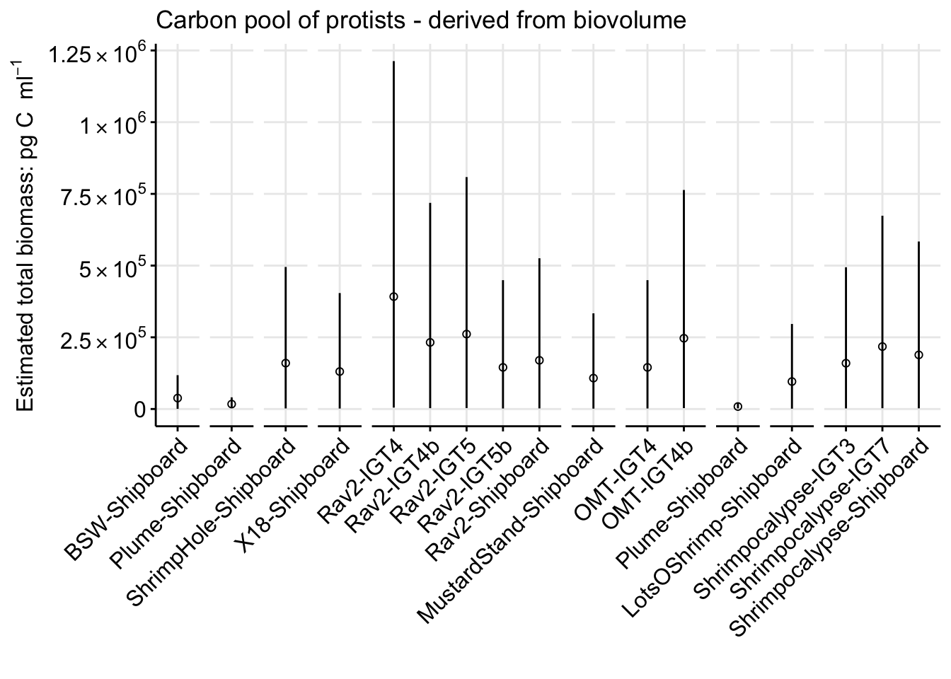

8.3 C biomass based on size fraction

Derived from Caron et al. 1995

1. Assign by size class

Assuming conversion factor is 183 fg C per um.

For nanoplankton <20um, picoplankton are included for now. We are assuming the size range of nanoplankton are 3um.

Code

vol_nano <- (4/3) * pi * (3^3)
vol_nano # units are um^3

[1] 113.0973

Code

fg_nano_c <- 183 * vol_nano #units are now fg per C
c_n <- (fg_nano_c)/1000
c_n

[1] 20.69681

For microplankton, we are assuming the cell diameter is 50 um.

Code

vol_micr <- (4/3) * pi * (50^3)
vol_micr # units are um^3

[1] 523598.8

Code

fg_micr_c <- 183 * vol_micr #units are now fg per C
c_m <- (fg_micr_c)/1000
c_m

[1] 95818.58

Code

c_n

[1] 20.69681

Code

c_m * (1e-6)

[1] 0.09581858

Code

# 1pg to 1e-6ug

Code

pgC_ml_sizefrac_bysample_tmp <- counts_cellsml_avg %>% 
  mutate(IGT_REP = case_when(
    IGT_REP == "Bag" ~ "Shipboard",
    TRUE ~ IGT_REP
  )) %>% 
  unite("Experiment_rep", Name, IGT_REP, sep = "-", remove = FALSE) %>% 
  filter(TimePoint == "T0") %>%
  filter(VARIABLE != "eukCONC") %>% # isolate micro vs. nano
  mutate(SAMPLE_TYPE_BIN = case_when(
    Name == "Background" ~ "Non-vent",
    Name == "Plume" ~ "Non-vent",
    TRUE ~ "Vent"
  )) %>% 
  mutate(pg_C_cell = case_when(
    VARIABLE == "microCONC" ~ c_m,
    VARIABLE == "nanoCONC" ~ c_n
  )) %>% 
  # multiply mean cells per ml of micro and nano by pg C for each size fraction:
  mutate(pg_C_ml_TMP = MEAN * pg_C_cell) %>% 
  group_by(Experiment_rep, Site, Name, TimePoint, EXP_TYPE, IGT_REP, SAMPLE_TYPE_BIN, VARIABLE) %>% 
  # Take the average of the micro and nano for each experiment.
  summarise(pg_C_ml = mean(pg_C_ml_TMP))

`summarise()` has grouped output by 'Experiment_rep', 'Site', 'Name',
'TimePoint', 'EXP_TYPE', 'IGT_REP', 'SAMPLE_TYPE_BIN'. You can override using
the `.groups` argument.

Code

# Isolate total euk for each experiment by adding.
tmp2 <- pgC_ml_sizefrac_bysample_tmp %>% 
  group_by(Experiment_rep, Site, Name, TimePoint, EXP_TYPE, IGT_REP, SAMPLE_TYPE_BIN) %>% 
  # Add across micro and nano to get total
  summarize(pg_C_ml = sum(pg_C_ml)) %>% 
  add_column(VARIABLE = "totaleuk")

`summarise()` has grouped output by 'Experiment_rep', 'Site', 'Name',
'TimePoint', 'EXP_TYPE', 'IGT_REP'. You can override using the `.groups`
argument.

Code

pgC_ml_sizefrac_bysample <- rbind(tmp2, pgC_ml_sizefrac_bysample_tmp)
pgC_ml_sizefrac_bysample

# A tibble: 51 × 9
# Groups:   Experiment_rep, Site, Name, TimePoint, EXP_TYPE, IGT_REP [17]
   Experiment_rep Site  Name  TimePoint EXP_TYPE IGT_REP SAMPLE_TYPE_BIN pg_C_ml
   <chr>          <chr> <chr> <chr>     <chr>    <chr>   <chr>             <dbl>
 1 BSW-Shipboard  VD    BSW   T0        Bag      Shipbo… Vent             1.90e3
 2 LotsOShrimp-S… Picc… Lots… T0        Bag      Shipbo… Vent             4.78e3
 3 MustardStand-… VD    Must… T0        Bag      Shipbo… Vent             5.38e3
 4 OMT-IGT4       VD    OMT   T0        IGT      IGT4    Vent             6.71e6
 5 OMT-IGT4b      VD    OMT   T0        IGT      IGT4b   Vent             1.34e7
 6 Plume-Shipboa… Picc… Plume T0        Bag      Shipbo… Non-vent         8.95e5
 7 Plume-Shipboa… VD    Plume T0        Bag      Shipbo… Non-vent         2.19e6
 8 Rav2-IGT4      VD    Rav2  T0        IGT      IGT4    Vent             1.96e4
 9 Rav2-IGT4b     VD    Rav2  T0        IGT      IGT4b   Vent             3.36e6
10 Rav2-IGT5      VD    Rav2  T0        IGT      IGT5    Vent             6.72e6
# ℹ 41 more rows
# ℹ 1 more variable: VARIABLE <chr>

Code

pgC_ml_sizefrac_bysample %>% 
  group_by(SAMPLE_TYPE_BIN, VARIABLE) %>% 
  summarise(MEAN_pg_C_ml = mean(pg_C_ml),
            MAX_pg_C_ml = max(pg_C_ml),
            MIN_pg_C_ml = min(pg_C_ml))

`summarise()` has grouped output by 'SAMPLE_TYPE_BIN'. You can override using
the `.groups` argument.

# A tibble: 6 × 5
# Groups:   SAMPLE_TYPE_BIN [2]
  SAMPLE_TYPE_BIN VARIABLE  MEAN_pg_C_ml MAX_pg_C_ml MIN_pg_C_ml
  <chr>           <chr>            <dbl>       <dbl>       <dbl>
1 Non-vent        microCONC     1542774.    2191604.     893944.
2 Non-vent        nanoCONC         2120.       2792.       1448.
3 Non-vent        totaleuk      1544894.    2194397.     895392.
4 Vent            microCONC     3559014.   13409159.          0 
5 Vent            nanoCONC         8180.      19551.       1901.
6 Vent            totaleuk      3567194.   13418572.       1901.

Code

by_sizefrac_plot <- pgC_ml_sizefrac_bysample %>% 
   mutate(NameOrder = factor(Name, levels = vent_ids, labels = vent_fullname)) %>%
  mutate(SiteOrder = factor(Site, levels = site_ids, labels = site_fullname)) %>% 
  ggplot(aes(x = Experiment_rep, y = (pg_C_ml))) +
    geom_point(color = "black", aes(shape = VARIABLE)) + 
    # geom_linerange(aes(ymin = (pgC_ml_min/1000), ymax = (pgC_ml_max/1000))) +
  facet_grid(.~SiteOrder + NameOrder, space = "free", scales = "free") +
  scale_y_continuous(labels = scientific_10) +
    theme_minimal() +
    theme(panel.grid.major = element_line(), panel.grid.minor = element_blank(),
           panel.background = element_blank(), 
           axis.line = element_line(colour = "black"), 
           axis.text.x = element_text(color="black", size = 12, 
                                      angle = 45, hjust = 1, vjust = 1), 
           axis.text.y = element_text(color="black", size = 12),
           axis.title =element_text(color="black", size = 12),
           axis.ticks = element_line(),
           strip.text =element_blank(), legend.title = element_blank())+
    guides(fill = guide_legend(override.aes = list(shape = c(21))),
       shape = guide_legend(override.aes = list(fill = "black"))) +
    labs(x = "", y = bquote("Estimated total biomass: pg C " ~ml^-1),
         title = "Carbon pool of protists - based on size fraction")

Combined supplementary plot showing two routes of determining total biomass.

8.4 Figure S3

Code

# svg("../../../Manuscripts_presentations_reviews/MCR-grazing-2023/svg-files-figures/figS3_new.svg", h = 8, w = 7)
by_biovol_plot + by_sizefrac_plot + patchwork::plot_layout(ncol = 1) +
  plot_annotation(tag_levels = "a")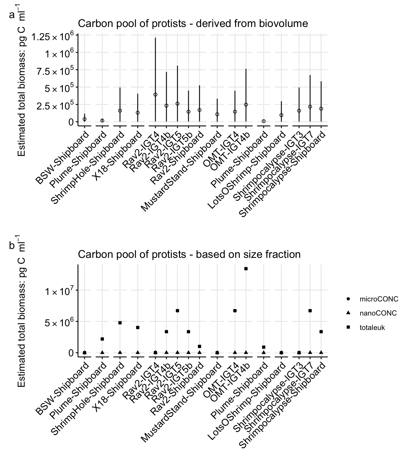

Code

# dev.off()

8.5 Compare total carbon biomass - euks

Compilation table of carbon biomass values for microeukaryotes by sample type and vent field

Table S4

Code

## Carbon biomass derived from biovolume, by vent field (vent only)
table4_cbiomass_total <- pgC_ml_biov_bysample %>% 
  group_by(VARIABLE, Site, EXP_TYPE, SAMPLE_TYPE_BIN) %>% 
  summarise(MEAN_pg_C_ml = mean(pgC_ml_mean),
            MAX_pg_C_ml = max(pgC_ml_mean),
            MIN_pg_C_ml = min(pgC_ml_mean)) %>% 
  add_column(ORIGIN = "bybiovolume") %>% 
  rbind(pgC_ml_sizefrac_bysample %>% 
  group_by(VARIABLE, Site, SAMPLE_TYPE_BIN, EXP_TYPE) %>% 
  summarise(MEAN_pg_C_ml = mean(pg_C_ml),
            MAX_pg_C_ml = max(pg_C_ml),
            MIN_pg_C_ml = min(pg_C_ml)) %>% 
  add_column(ORIGIN = "sizefrac")
  )

`summarise()` has grouped output by 'VARIABLE', 'Site', 'EXP_TYPE'. You can
override using the `.groups` argument.
`summarise()` has grouped output by 'VARIABLE', 'Site', 'SAMPLE_TYPE_BIN'. You
can override using the `.groups` argument.

Code

# table4_cbiomass_total
write.csv(table4_cbiomass_total, file = "output-data/tableS4-cbiomass.csv")

8.6 Compare biovolumes from literature to measured in this study

Compare with Menden-Deuer and Lessard 2000, Table 2 - using only the heterotrophic species measured. Based on Table 2, the min volume was 4745 and the maximum was 1.2 x10^7 µm^3. Carbon content was measured at pg per cell, this was 469.48-35,339 pg per cell.

Import the heterotroph species volume and carbon content to compare to my measured values. Compare to md-lessard (Supplementary)

Code

c_prev <- read.delim("input-data/md-lessard-2000.txt") # Table 2, heterotrophs only
# c_prev
# biov
# combine and plot
carbon_compare <- c_prev %>% 
  add_column(source = "Menden-Deuer Lessard") %>% 
  select(source, Volume = vol, pgC_cell) %>% 
  rbind(biov_calc %>% add_column(source = "MCR") %>% select(source, Volume = BIOVOLUME, pgC_cell = pgC_cell_MD_nodiatom)) %>% 
    ggplot(aes(x = Volume, y = pgC_cell, fill = source)) +
      geom_point(aes(fill = source), shape = 23, color = "black", size = 3) +
      scale_y_log10() + scale_x_log10() +
      labs(title = "Compare literature to measured cell volume & C content",
           x = bquote("Volume" ~µm^3),
           y = bquote("pg C" ~cell^-1)) +
      theme_bw() + theme(legend.title = element_blank(),
                         axis.title = element_text(size = 14),
                         axis.text = element_text(size = 14),
                         legend.text = element_text(size = 14))

carbon_compare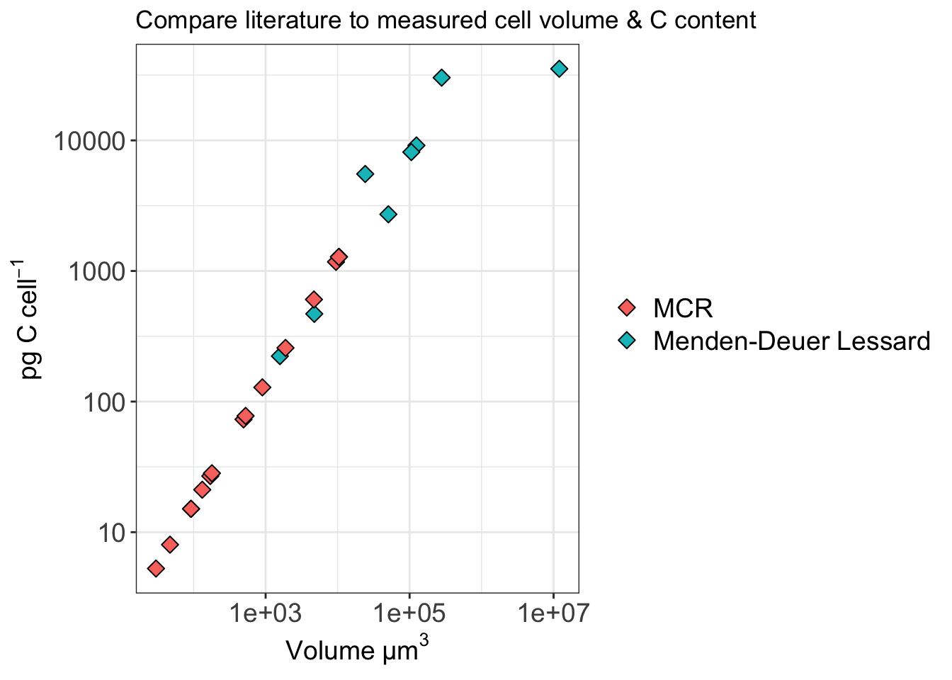

Upon comparison, the measured carbon content was much lower from the grazing experiments. This makes sense, as I am looking at preserved specimen and a smaller total number of cells. AND the deep-sea protist cell sizes may be smaller overall.

Code

# head(pgC_ml_biov_bysample)
# unique(pgC_ml_biov_bysample)

pgC_ml_biov_bysample %>% 
  unite("SITE_TYPE", Site, EXP_TYPE, sep = "-", remove = FALSE) %>% 
  ggplot(aes(y = pgC_ml_mean, x = SAMPLE_TYPE_BIN, shape = SITE_TYPE, 
             fill = SITE_TYPE, color = SITE_TYPE)) +
  geom_boxplot() +
  geom_jitter(stat = "identity", aes(shape = SITE_TYPE, 
                                     fill = SITE_TYPE, color = SITE_TYPE),
              stroke = 2, size = 3, width = 0.25) +
    scale_shape_manual(values = c(21, 21, 21, 21)) +
    scale_fill_manual(values = c("white", "#264653", "white", "#E76F51")) +
    scale_color_manual(values = c("#264653", "#264653", "#E76F51", "#E76F51")) +
  # facet_grid(.~FIELDORDER, space = "free", scales = "free") +
  # coord_flip() +
    theme_minimal() +
    theme(panel.grid.major = element_line(), panel.grid.minor = element_blank(),
           panel.background = element_blank(), 
           axis.line = element_line(colour = "black"), 
           axis.text.x = element_text(color="black", size = 13, 
                                      angle = 45, hjust = 1, vjust = 1), 
           axis.text.y = element_text(color="black", size = 13),
           axis.title =element_text(color="black", size = 13),
           axis.ticks = element_line(),
           strip.text =element_blank(), legend.title = element_blank(),
          legend.position = "top") +
    labs(x = "", y = bquote("pg C " ~ml^-1))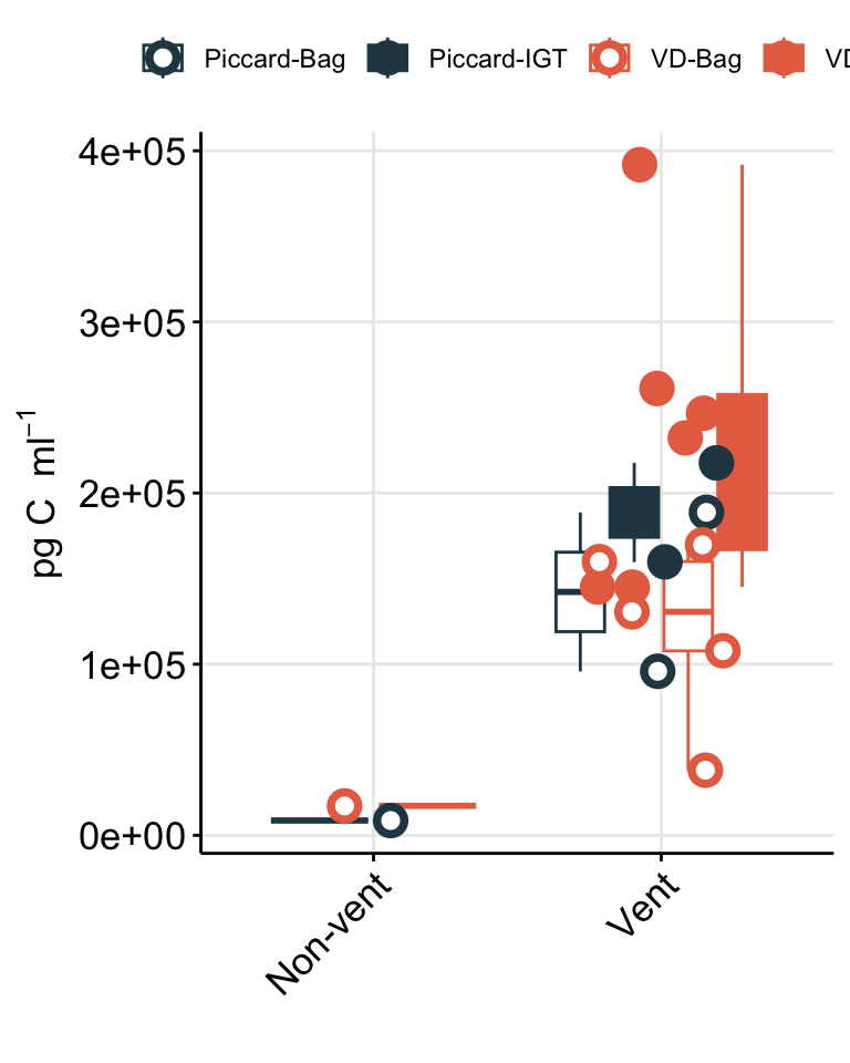

9 Carbon biomass for prokaryotes

Now, report estimated carbon per cell for bacteria.

Units: fg C per cell.

Code

bac_carbon_Mor_fg <- (86) 
#From Derived from Morono et al. 2011 

bac_carbon_Lof_fg <- (173) 
# Derived from McNichol et al. 2018; LOFERER-KROBACHER, J. KLIMA & R. PSENNER 1998

# fg C per cell
bac_carbon_mean <- 15
bac_carbon_min <- 10
bac_carbon_max <- 20

Import main table with all estimates of cells

Code

# table_wcalcs <- read_delim(file = "output-data/table1-grazing-exp-list.txt", delim = "\t")
# head(table_wcalcs)

RATE_min units = FLPs per grazer per minute Clearance rate _ml = ml per grazer per hour

Code

##
est_prok_carbon <- table_wcalcs %>% 
  select(SiteOrder, NameOrder, SiteOrder, FLUID_ORIGIN, CRUISE_SAMPLE,  starts_with("PROK_"), GRAZING_EFFECT_hr, CLEARANCE_RATE_ml, RATE_minute) %>% 
  # Add in calcs by fg C per cell.
  ## Estimates of carbon pool of microbes per ml. 
  mutate(MOR_fgC_ml = bac_carbon_Mor_fg * PROK_ml,
         LOF_fgC_ml = bac_carbon_Lof_fg * PROK_ml,
         MEAN_fgC_ml = bac_carbon_mean * PROK_ml,
         MAX_fgC_ml = bac_carbon_max * PROK_ml,
         MIN_fgC_ml = bac_carbon_min * PROK_ml) %>% 
  pivot_longer(cols = ends_with("fgC_ml"), names_to = "prokC_category", values_to = "fgC_ml")

# head(est_prok_carbon)

Get summary of prokaryotic biomass

Code

est_prok_carbon %>% 
  mutate(SAMPLE_TYPE_BIN = case_when(
    NameOrder == "Background" ~ "Non-vent",
    NameOrder == "Plume" ~ "Non-vent",
    TRUE ~ "Vent"
  )) %>%
  group_by(SAMPLE_TYPE_BIN, prokC_category) %>% 
  # 1 fg == 0.001 pg
  # Convert to pg C per ml
  summarise(mean_pgC_ml = mean((fgC_ml)*(0.001)),
            min_pgC_ml = min((fgC_ml)*(0.001)),
            max_pgC_ml = max((fgC_ml)*(0.001))) 

`summarise()` has grouped output by 'SAMPLE_TYPE_BIN'. You can override using
the `.groups` argument.

# A tibble: 10 × 5
# Groups:   SAMPLE_TYPE_BIN [2]
   SAMPLE_TYPE_BIN prokC_category mean_pgC_ml min_pgC_ml max_pgC_ml
   <chr>           <chr>                <dbl>      <dbl>      <dbl>
 1 Non-vent        LOF_fgC_ml           6101.      2851.      8897.
 2 Non-vent        MAX_fgC_ml            705.       330.      1029.
 3 Non-vent        MEAN_fgC_ml           529.       247.       771.
 4 Non-vent        MIN_fgC_ml            353.       165.       514.
 5 Non-vent        MOR_fgC_ml           3033.      1417.      4423.
 6 Vent            LOF_fgC_ml          19884.      7263.     41276.
 7 Vent            MAX_fgC_ml           2299.       840.      4772.
 8 Vent            MEAN_fgC_ml          1724.       630.      3579.
 9 Vent            MIN_fgC_ml           1149.       420.      2386.
10 Vent            MOR_fgC_ml           9885.      3611.     20519.

Code

# head(est_prok_carbon)

9.1 Incorporate carbon biomass of prey and grazing rate

Clearance rate is mL per grazer per hour (Table S3). Grazing effect is prokaryotes ml-1 hr-1 (Table S3).

Code

## Carbon consumed based on clearance rate
carbon_consumed <- est_prok_carbon %>% 
  #use only value from Morono et al., convert to pg C per cell.
  filter(prokC_category == "MOR_fgC_ml") %>% 
  add_column(bac_carbon_Mor_pg = (bac_carbon_Mor_fg * 0.001)) %>% 
  select(SiteOrder, NameOrder, SiteOrder, FLUID_ORIGIN, CRUISE_SAMPLE, PROK_ml, GRAZING_EFFECT_hr, CLEARANCE_RATE_ml, bac_carbon_Mor_pg, fgC_ml) %>% 
  # Clearance rate * fg of prok == pg C per grazer per hr
  # bac_carbon_Mor_pg * grazing effect == pg C per ml per hr
  mutate(pgC_pergrazer_CLEARANCE = (fgC_ml*0.001) * CLEARANCE_RATE_ml,
         pgC_perml_perhr = bac_carbon_Mor_pg * GRAZING_EFFECT_hr)
carbon_consumed

# A tibble: 14 × 11
   SiteOrder NameOrder      FLUID_ORIGIN CRUISE_SAMPLE PROK_ml GRAZING_EFFECT_hr
   <fct>     <fct>          <chr>        <chr>           <dbl>             <dbl>
 1 Piccard   Lots 'O Shrimp J2-1241      LV24           53878                0  
 2 Piccard   Plume          CTD004       Niskin 10      51429               44.3
 3 Piccard   Shrimpocalypse J2-1240      LV13          238590             6007. 
 4 Von Damm  Background     CTD002       Niskins 8-10   37890              127. 
 5 Von Damm  Mustard Stand  J2-1243      LV17           56677                0  
 6 Von Damm  Plume          CTD001       Niskin 2       16478               24.0
 7 Von Damm  Ravelin #2     J2-1238      LV13a          71147.             117. 
 8 Von Damm  Shrimp Hole    J2-1244      LV13           41983                0  
 9 Von Damm  X-18           J2-1235      LV23 & Bio5   111430             1166. 
10 Piccard   Shrimpocalypse J2-1240      IGT3          238590            17285. 
11 Von Damm  Old Man Tree   J2-1238      IGT4           71147.            1050. 
12 Von Damm  Ravelin #2     J2-1244      IGT4           71147.           15867. 
13 Von Damm  Ravelin #2     J2-1244      IGT5           71147.               0  
14 <NA>      <NA>           <NA>         <NA>          238590               NA  
# ℹ 5 more variables: CLEARANCE_RATE_ml <dbl>, bac_carbon_Mor_pg <dbl>,
#   fgC_ml <dbl>, pgC_pergrazer_CLEARANCE <dbl>, pgC_perml_perhr <dbl>

10 Environmental parameters - MCR

Import from Hu et al. (Molecular Ecology).

Code

env_tmp <- read.delim("../../microeuks_deepbiosphere_datamine/microeuk-amplicon-survey/data-input/samplelist-metadata.txt")
# head(env_tmp)

mcr_metadata <- env_tmp %>% 
  filter(SITE == "VonDamm" | SITE  == "Piccard") %>% 
  mutate(FIELD =  case_when(
    SITE == "VonDamm"  ~ "Von Damm",
    SITE == "Piccard" ~ "Piccard")) %>% 
  filter(SAMPLETYPE != "Incubation") %>% 
  separate(SAMPLE, into = c("num", "loc", "loc2", "fluid_origin", "name", "FLUID_ORIGIN", "else"), remove = FALSE) %>% 
  select(-Sample_or_Control, -SAMPLEID, -ref_num, -SITE, SEQ_SAMPLE = SAMPLE,FLUID_ORIGIN, everything(), -num, -loc, -loc2, -fluid_origin, -name, -`else`)

Warning: Expected 7 pieces. Additional pieces discarded in 16 rows [2, 3, 4, 5, 6, 7, 8,
9, 10, 11, 12, 13, 14, 15, 16, 17].

Warning: Expected 7 pieces. Missing pieces filled with `NA` in 1 rows [1].

Code

# View(mcr_metadata)

Generate supplementary table.

Code

supp_table_env_mcr <- mcr_metadata %>% 
  select(FIELD, VENT, SAMPLETYPE, DEPTH, TEMP = temp, PH = pH, PERCSEA = percseawater, MG = mg, H2 = h2, H2S = h2s, CH4 = ch4, MICROBIAL = ProkConc, everything())

# Save supplementary metadata table:
# write.csv(supp_table_env_mcr, file = "output-data/supp_table_MCR_metadata.csv")

11 Analysis of grazing rate results

Re-import table from output table with all grazing values

Format and factor values to plot, and prioritize these values:

• Grazing rate column == FLP per minute consumed
• Grazing effect hr == cells per ml per hr
• Specific ingestion rate == % of cell carbon per day, estimated with literature and measured carbon values

Report grazing rates

Code

# head(table_wcalcs)
# head(table_grazerate_wflp_wprok_weuk)
# head(pgC_ml_biov_bysample)
# head(pgC_ml_sizefrac_bysample)


# save(table_grazerate_wflp_wprok_weuk, table_wcalcs, pgC_ml_biov_bysample, pgC_ml_sizefrac_bysample, carbon_consumed, file = "output-data/processed-dfs-mcr-grazing.RData")
# load("output-data/processed-dfs-mcr-grazing.RData")

Plot grazing rates

Code

grazing_rate <- table_wcalcs %>%
  mutate(SAMPLE_TYPE_BIN = case_when(
    NameOrder == "Background" ~ "Non-vent",
    NameOrder == "Plume" ~ "Non-vent",
    TRUE ~ "Vent"
  )) %>%
  mutate(NameOrder = factor(Name, levels = vent_ids, labels = vent_fullname)) %>%
  mutate(SiteOrder = factor(FIELD, levels = site_ids, labels = site_fullname)) %>% 
  # group_by(SAMPLE_TYPE_BIN) %>%
  separate(Experiment_rep, into = c("name", "exptype_rep"), remove = FALSE) %>% 
  mutate(exptype = case_when(exptype_rep == "Shipboard" ~ "Shipboard",
                             TRUE ~ "IGT")) %>% 
  ggplot(aes(x = NameOrder, y = GRAZING_EFFECT_hr, shape = SITE_TYPE, 
                                      fill = SITE_TYPE, color = SITE_TYPE)) +
  geom_errorbar(aes(ymax = (GRAZING_EFFECT_hr_max), ymin = (GRAZING_EFFECT_hr_min)), 
                  width = 0.2, color = "black", position = position_dodge(width = 0.25)) +
    geom_point(stat = "identity", aes(shape = SITE_TYPE, 
                                      fill = SITE_TYPE, color = SITE_TYPE),
               stroke = 2, size = 3, position = position_dodge(width = 0.25)) +
  scale_shape_manual(values = c(21, 21, 21, 21)) +
  scale_fill_manual(values = c("white", "#264653", "white", "#E76F51")) +
  scale_color_manual(values = c("#264653", "#264653", "#E76F51", "#E76F51")) +
  facet_grid(.~SiteOrder, space = "free", scales = "free") +
  theme_minimal() +
  theme(panel.grid.major = element_line(), panel.grid.minor = element_blank(),
        panel.background = element_blank(), 
        axis.line = element_line(colour = "black"), 
        axis.text.x = element_text(color="black", size = 13, 
                                   angle = 45, hjust = 1, vjust = 1), 
        axis.text.y = element_text(color="black", size = 13),
        axis.title =element_text(color="black", size = 13),
        axis.ticks = element_line(),
        strip.text =element_blank(), legend.title = element_blank(),
        legend.position = "top") +
  labs(x = "", y = bquote("Cells consumed " ~ml^-1 ~hr^-1))

grazing_rate + scale_y_log10()

Warning: Transformation introduced infinite values in continuous y-axis
Transformation introduced infinite values in continuous y-axis
Transformation introduced infinite values in continuous y-axis
Transformation introduced infinite values in continuous y-axis

Warning: Removed 1 rows containing missing values (`geom_point()`).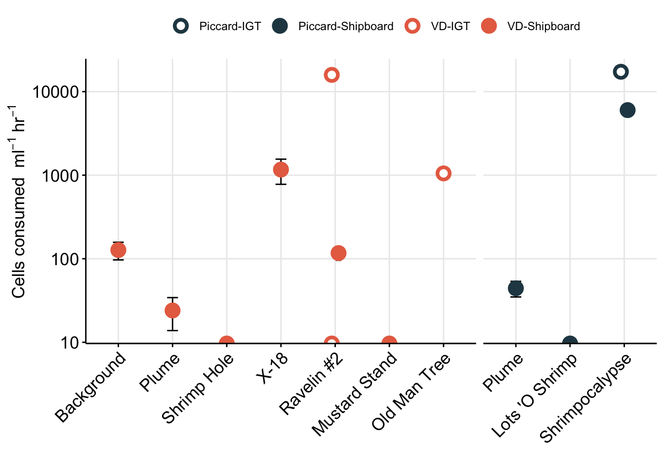

Code

grazing_rate + scale_y_continuous(labels = scientific_10)

Warning: Removed 1 rows containing missing values (`geom_point()`).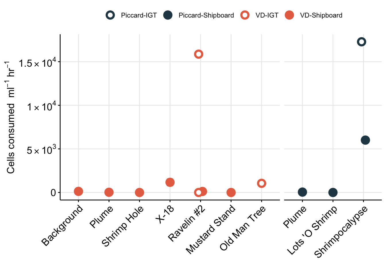

Code

grazing_rate + scale_y_log10(labels = scientific_10, limits = c(1,1e5))

Warning: Transformation introduced infinite values in continuous y-axis
Transformation introduced infinite values in continuous y-axis
Transformation introduced infinite values in continuous y-axis
Transformation introduced infinite values in continuous y-axis

Warning: Removed 1 rows containing missing values (`geom_point()`).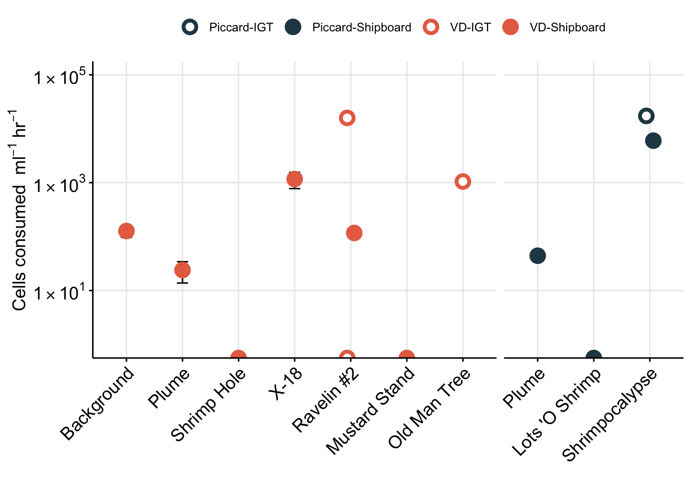

Box plots: Grazing rate

Code

boxplot_rate_site <- table_wcalcs %>%
  mutate(SAMPLE_TYPE_BIN = case_when(
    NameOrder == "Background" ~ "Non-vent",
    NameOrder == "Plume" ~ "Non-vent",
    TRUE ~ "Vent"
  )) %>%
  mutate(NameOrder = factor(Name, levels = vent_ids, labels = vent_fullname)) %>%
  mutate(SiteOrder = factor(FIELD, levels = site_ids, labels = site_fullname)) %>% 
  # group_by(SAMPLE_TYPE_BIN) %>%
  separate(Experiment_rep, into = c("name", "exptype_rep"), remove = FALSE) %>% 
  mutate(exptype = case_when(exptype_rep == "Shipboard" ~ "Shipboard",
                             TRUE ~ "IGT")) %>% 
  ggplot(aes(x = SAMPLE_TYPE_BIN, y = GRAZING_EFFECT_hr, color = SiteOrder)) +
    geom_boxplot(aes(color = SiteOrder)) +
  geom_jitter(stat = "identity", size = 2, width = 0.3, stroke = 2, shape = 21, aes(color = SiteOrder, fill = SiteOrder)) +
  scale_fill_manual(values = c("#264653", "#E76F51")) +
  scale_color_manual(values = c("#264653", "#E76F51")) +
  coord_flip() +
  facet_grid(.~SiteOrder) +
  theme_minimal() +
  scale_y_log10(position = "right") +
  theme(panel.grid.major = element_line(), panel.grid.minor = element_blank(),
        panel.background = element_blank(), 
        axis.line = element_line(colour = "black"), 
        axis.text.x = element_text(color="black", size = 10, 
                                   angle = 0, hjust = 0.5, vjust = 0), 
        axis.text.y = element_text(color="black", size = 12),
        axis.title =element_text(color="black", size = 12),
        axis.ticks = element_line(),
        strip.text =element_blank(), legend.title = element_blank()) +
  labs(x = "", y = bquote("Cells consumed " ~ml^-1 ~hr^-1))

Code

boxplot_rate_exp <- table_wcalcs %>%
  mutate(SAMPLE_TYPE_BIN = case_when(
    NameOrder == "Background" ~ "Non-vent",
    NameOrder == "Plume" ~ "Non-vent",
    TRUE ~ "Vent"
  )) %>%
  mutate(NameOrder = factor(Name, levels = vent_ids, labels = vent_fullname)) %>%
  mutate(SiteOrder = factor(FIELD, levels = site_ids, labels = site_fullname)) %>% 
  separate(Experiment_rep, into = c("name", "exptype_rep"), remove = FALSE) %>% 
  mutate(exptype = case_when(exptype_rep == "Shipboard" ~ "Shipboard",
                             TRUE ~ "IGT")) %>% 
  filter(SAMPLE_TYPE_BIN == "Vent") %>% 
  ggplot(aes(x = exptype, y = GRAZING_EFFECT_hr)) +
    geom_boxplot() +
  geom_jitter(stat = "identity", size = 2, width = 0.3, stroke = 2, aes(shape = exptype)) +
  scale_shape_manual(values = c(21, 19)) + 
  coord_flip() +
  # facet_grid(.~SiteOrder) +
  theme_minimal() +
  scale_y_log10(position = "right") +
  theme(panel.grid.major = element_line(), panel.grid.minor = element_blank(),
        panel.background = element_blank(), 
        axis.line = element_line(colour = "black"), 
        axis.text.x = element_text(color="black", size = 10, 
                                   angle = 0, hjust = 0.5, vjust = 0), 
        axis.text.y = element_text(color="black", size = 12),
        axis.title =element_text(color="black", size = 12),
        axis.ticks = element_line(),
        strip.text =element_blank(), legend.title = element_blank()) +
  labs(x = "", y = bquote("Cells consumed " ~ml^-1 ~hr^-1))

12 Figure 1 compilation

Code

# svg("../../../Manuscripts_presentations_reviews/MCR-grazing-2023/svg-files-figures/fig1.svg", w = 10, h = 8)

  (euk_plot + theme(legend.position = "none")) +
  (prok_plot + theme(legend.position = "none")) +
  grazing_min_plot + theme(legend.position = "none") +
  # (grazing_min_plot + theme(legend.position = "none") + scale_y_continuous(limits = c(0, 0.02))) +
  (grazing_rate + scale_y_log10(labels = scientific_10, limits = c(1,1e5)) + theme(legend.position = "none")) + patchwork::plot_layout(ncol = 2) +
  patchwork::plot_annotation(tag_levels = "a")

Warning: Transformation introduced infinite values in continuous y-axis
Transformation introduced infinite values in continuous y-axis
Transformation introduced infinite values in continuous y-axis
Transformation introduced infinite values in continuous y-axis

Warning: Removed 1 rows containing missing values (`geom_point()`).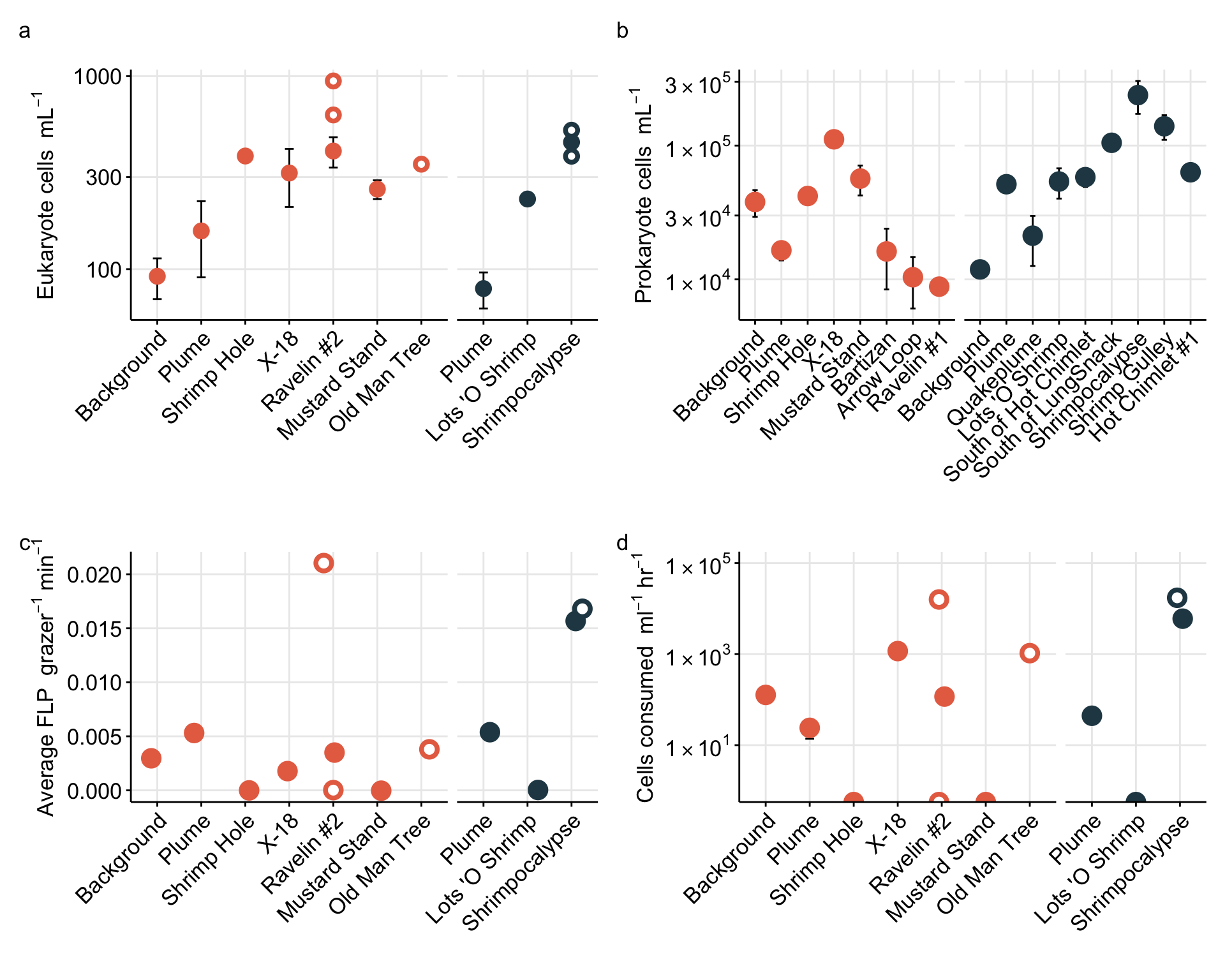

Code

# dev.off()

Code

# svg("../../../Manuscripts_presentations_reviews/MCR-grazing-2023/svg-files-figures/fig1-revisions.svg", w = 11, h = 6)
(boxplot_eukcell_site + theme(legend.position = "none")) + 
  (boxplot_rate_site + theme(legend.position = "none",  axis.text.y = element_blank())) +
  (boxplot_eukcell_exp + theme(legend.position = "none")) + 
  (boxplot_rate_exp + theme(legend.position = "none",  axis.text.y = element_blank())) +
     patchwork::plot_layout(ncol = 2) +
  patchwork::plot_annotation(tag_levels = "a") & theme(plot.tag = element_text(size = 16))

Warning: Transformation introduced infinite values in continuous y-axis
Transformation introduced infinite values in continuous y-axis

Warning: Removed 5 rows containing non-finite values (`stat_boxplot()`).

Warning: Removed 1 rows containing missing values (`geom_point()`).

Warning: Transformation introduced infinite values in continuous y-axis
Transformation introduced infinite values in continuous y-axis

Warning: Removed 5 rows containing non-finite values (`stat_boxplot()`).

Warning: Removed 1 rows containing missing values (`geom_point()`).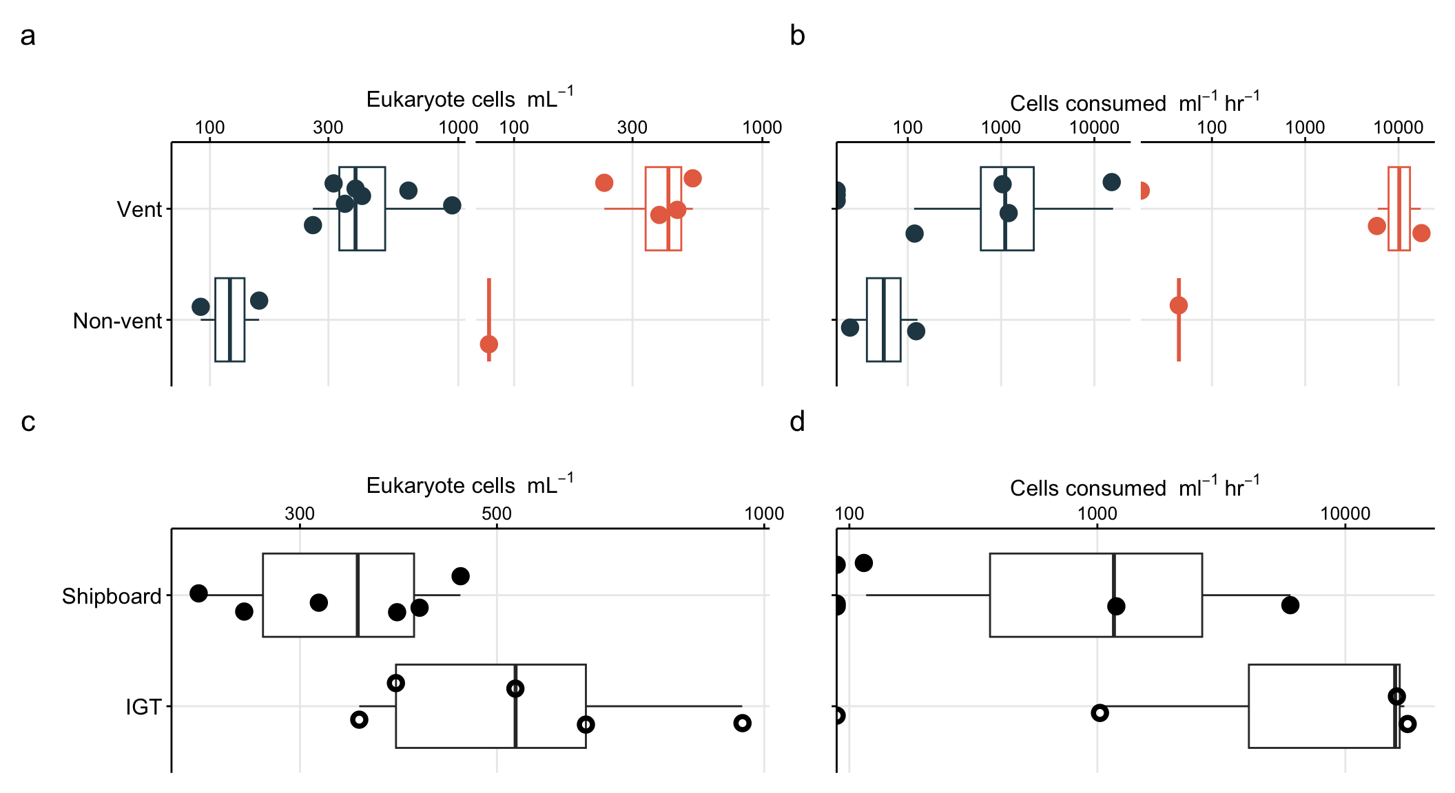

Code

# dev.off()

12.1 Grazing rate vs. cells ml

Combine metadata from environment with grazing rate results.

Code

# head(table_wcalcs)
# View(mcr_metadata)
# Modify fluid origin to match metadata and results
mod_metadata <- mcr_metadata %>% 
  filter(SAMPLETYPE != "Incubation") %>%
  filter(VENT != "Quakeplume") %>% 
  separate(FLUID_ORIGIN, into = c("FLUID", "HOG"), sep = "HOG", remove = FALSE) %>% 
  separate(FLUID_ORIGIN, into = c("FLUID2", "excess"), sep = "J2", remove = FALSE) %>% 
  separate(excess, into = c("FLUID3", "hogexcess"), sep = "HOG", remove = FALSE) %>% 
  mutate(FLUID_ORIGIN = case_when(
    FLUID2 == "CTD003" ~ "CTD001", #Correction for plume VD
    is.na(FLUID3) ~ FLUID2,
    TRUE ~ paste("J2-", FLUID3, sep = "")
  )) %>% 
  select(-FLUID, -FLUID2, -FLUID3, -HOG, -excess, -hogexcess) %>% 
  mutate(Name = case_when(
    VENT == "OldManTree" ~ "OMT",
    TRUE ~ VENT
  ))

Warning: Expected 2 pieces. Missing pieces filled with `NA` in 4 rows [1, 2, 6, 7].
Expected 2 pieces. Missing pieces filled with `NA` in 4 rows [1, 2, 6, 7].

Code

# unique(table_wcalcs$Name)
# mod_metadata
# setdiff(mod_metadata$FLUID_ORIGIN, table_wcalcs$FLUID_ORIGIN)

grazing_wenv <- table_wcalcs %>% 
  select(SiteOrder, Name, Experiment_rep, FLUID_ORIGIN, RATE_minute, starts_with("EUK_"), starts_with("PROK_"), starts_with("GRAZING_EFFECT"), CLEARANCE_RATE_ml, SPEC_GRAZE_RATE_hr, BAC_TURNOVER_PERC) %>%
  left_join(mod_metadata, join_by(Name == Name, FLUID_ORIGIN == FLUID_ORIGIN))

# View(grazing_wenv)

Code

# View(plot_metadata)
euk_temp <- grazing_wenv %>% 
    mutate(TEMP = as.numeric(temp)) %>% 
    mutate(EXP_TYPE = case_when(
      grepl("IGT", Experiment_rep) ~ "IGT",
      TRUE ~ "Shipboard"
    )) %>% 
  unite(SITE_TYPE, SiteOrder, EXP_TYPE, sep = "-", remove = FALSE) %>% 
  filter(!(SITE_TYPE == "NA-IGT")) %>% 
  ggplot(aes(x = GRAZING_EFFECT_hr, y = EUK_ml, 
             fill = TEMP, color = TEMP, shape = SITE_TYPE)) +
    # geom_errorbar(aes(ymin = (log10(EUK_ml)-(EUK_sem)),ymax = (log10(EUK_ml)+(EUK_sem)))) +
    #   geom_errorbarh(aes(xmin = log10(GRAZING_EFFECT_hr_min),xmax = log10(GRAZING_EFFECT_hr_max))) +
  geom_errorbar(aes(ymin = ((EUK_ml)-(EUK_sem)),ymax = ((EUK_ml)+(EUK_sem))), color = "black") +
      geom_errorbarh(aes(xmin = (GRAZING_EFFECT_hr_min),xmax = (GRAZING_EFFECT_hr_max)), color = "black") +
  # geom_point(aes(shape = EXP_TYPE), size = 4, stroke = 2) +
  geom_point(aes(shape = SITE_TYPE), size = 4, stroke = 2) +
  scale_y_log10() + 
  scale_x_log10() +
  scale_shape_manual(values = c(2, 24, 6, 25)) +
  scale_fill_distiller(palette = "YlOrRd", direction=2, na.value = "grey50") +
  scale_color_distiller(palette = "YlOrRd", direction=2, na.value = "grey50") +
  theme_minimal() +
    theme(rect = element_rect(fill = "transparent"),
        # panel.background = element_rect(fill = "transparent"),
        panel.background = element_rect(fill = "#f0f0f0"),
        plot.background = element_rect(fill = "transparent", color = NA),
        panel.grid.major = element_line(color = "#737373"), panel.grid.minor = element_blank(),
           axis.line = element_line(colour = "black"), 
           axis.text.x = element_text(color="black", size = 13), 
           axis.text.y = element_text(color="black", size = 13),
           axis.title =element_text(color="black", size = 13),
           axis.ticks = element_line(),
           strip.text =element_blank(), legend.title = element_blank()) +
  labs(x = bquote("Cells consumed "~mL^-1 ~hr^-1), y = bquote("Eukaryote cells "~mL^-1),
       title = "")

euk_temp

Warning: Transformation introduced infinite values in continuous x-axis
Transformation introduced infinite values in continuous x-axis
Transformation introduced infinite values in continuous x-axis
Transformation introduced infinite values in continuous x-axis
Transformation introduced infinite values in continuous x-axis

Warning: Removed 6 rows containing missing values (`geom_errorbarh()`).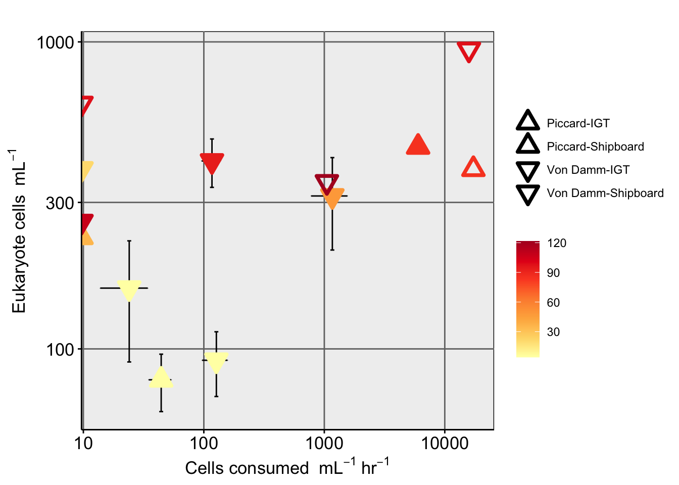

Code

prok_temp <- grazing_wenv %>% 
    mutate(TEMP = as.numeric(temp)) %>% 
    mutate(EXP_TYPE = case_when(
      grepl("IGT", Experiment_rep) ~ "IGT",
      TRUE ~ "Shipboard"
    )) %>% 
  unite(SITE_TYPE, SiteOrder, EXP_TYPE, sep = "-", remove = FALSE) %>% 
    filter(!(SITE_TYPE == "NA-IGT")) %>% 
  ggplot(aes(x = GRAZING_EFFECT_hr, y = PROK_ml, 
             fill = TEMP, color = TEMP, shape = SITE_TYPE)) +
  geom_errorbar(aes(ymin = ((PROK_ml)-(PROK_sem)),ymax = ((PROK_ml)+(PROK_sem))), color = "black") +
      geom_errorbarh(aes(xmin = (GRAZING_EFFECT_hr_min),xmax = (GRAZING_EFFECT_hr_max)), color = "black") +
  geom_point(aes(shape = SITE_TYPE), size = 4, stroke = 2) +
  scale_y_log10(labels = scientific_10) + 
  scale_x_log10() +
  # scale_shape_manual(values = c(1, 19)) +
  scale_shape_manual(values = c(2, 24, 6, 25)) +
  scale_fill_distiller(palette = "YlOrRd", direction=2, na.value = "grey50") +
  scale_color_distiller(palette = "YlOrRd", direction=2, na.value = "grey50") +
  theme_minimal() +
    theme(rect = element_rect(fill = "transparent"),
        # panel.background = element_rect(fill = "transparent"),
       panel.background = element_rect(fill = "#f0f0f0"),
        plot.background = element_rect(fill = "transparent", color = NA),
        panel.grid.major = element_line(color = "#737373"), panel.grid.minor = element_blank(),
           axis.line = element_line(colour = "black"), 
           axis.text.x = element_text(color="black", size = 13), 
           axis.text.y = element_text(color="black", size = 13),
           axis.title =element_text(color="black", size = 13),
           axis.ticks = element_line(),
           strip.text =element_blank(), legend.title = element_blank()) +
  labs(x = bquote("Cells consumed "~mL^-1 ~hr^-1), y = bquote("Microbial prey cells "~mL^-1),
       title = "")

prok_temp

Warning: Transformation introduced infinite values in continuous x-axis
Transformation introduced infinite values in continuous x-axis
Transformation introduced infinite values in continuous x-axis
Transformation introduced infinite values in continuous x-axis
Transformation introduced infinite values in continuous x-axis

Warning: Removed 6 rows containing missing values (`geom_errorbarh()`).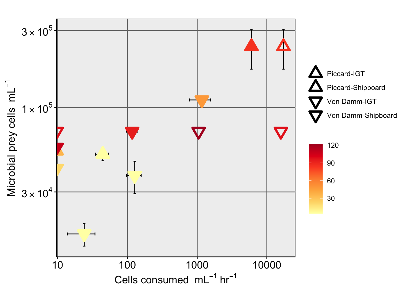

13 Figure 2 compilation

Code

# fig2 <- (euk_temp + labs(x = "") + theme(legend.position = "none")) + prok_temp + patchwork::plot_layout(ncol = 1) + patchwork::plot_annotation(tag_levels = "a")
# 
# svg("../../../Manuscripts_presentations_reviews/MCR-grazing-2023/svg-files-figures/fig2.svg", h = 10, w = 7)
# fig2
# dev.off()
# # 
# svg("../../../Manuscripts_presentations_reviews/MCR-grazing-2023/svg-files-figures/fig2-a.svg", h = 5, w = 7)
# euk_temp
# dev.off()
# 
# svg("../../../Manuscripts_presentations_reviews/MCR-grazing-2023/svg-files-figures/fig2-b.svg", h = 5, w = 7)
# prok_temp
# dev.off()

14 Comparison with Gorda Ridge

Import data from Gorda Ridge

Code

gr <- read.delim("../../GordaRidgeCruise_2019/protist-gordaridge-2021/Grazing-at-GordaRidge-SKH-2021/data-input/Grazing-calc-wCarbon-results.txt")

temps <- read.delim("../../GordaRidgeCruise_2019/protist-gordaridge-2019-analysis/temperature-allvents.txt")

mcr_graze <- read.delim("output-data/table-wcalc.txt")
glimpse(mcr_graze)

Rows: 14
Columns: 38
$ Experiment_rep        <chr> "LotsOShrimp-Shipboard", "Plume-Shipboard", "Shr…
$ FIELD                 <chr> "Piccard", "Piccard", "Piccard", "VD", "VD", "VD…
$ Name                  <chr> "LotsOShrimp", "Plume", "Shrimpocalypse", "BSW",…
$ SiteOrder             <chr> "Piccard", "Piccard", "Piccard", "Von Damm", "Vo…
$ NameOrder             <chr> "Lots 'O Shrimp", "Plume", "Shrimpocalypse", "Ba…
$ FLUID_ORIGIN          <chr> "J2-1241", "CTD004", "J2-1240", "CTD002", "J2-12…
$ CRUISE_SAMPLE         <chr> "LV24", "Niskin 10", "LV13", "Niskins 8-10", "LV…
$ RATE                  <dbl> -0.007605829, 0.005362856, 0.015686872, 0.002958…
$ RATE_minute           <dbl> 0.000000000, 0.005362856, 0.015686872, 0.0029588…
$ FLP_ml                <dbl> 617.1496, 29650.4676, 17003.1000, 4861.8239, 660…
$ TimePoints            <chr> "0, 15, 20, 40", "0, 10, 15, 20, 40", "0, 10, 14…
$ EXP_REPS              <int> 3, 3, 3, 3, 2, 3, 3, 2, 2, 1, 1, 1, 1, NA
$ EXP_VOL               <dbl> 1.50, 2.00, 1.50, 2.00, 1.50, 2.00, 1.50, 1.50, …
$ CTRL_REPS             <int> 2, 2, 2, 2, 2, 2, 2, 2, 2, NA, NA, NA, NA, NA
$ CTRL_VOL              <dbl> 0.2, 0.5, 0.2, 0.5, 0.2, 1.0, 0.5, 0.2, 0.5, NA,…
$ SITE_TYPE             <chr> "Piccard-Shipboard", "Piccard-Shipboard", "Picca…
$ Experiment            <chr> "LotsOShrimp-Shipboard", "Plume-Shipboard", "Shr…
$ VARIABLE              <chr> "eukCONC", "eukCONC", "eukCONC", "eukCONC", "euk…
$ EUK_ml                <dbl> 230.910, 79.301, 454.820, 91.838, 259.770, 157.7…
$ EUK_MinMax            <chr> "230.9 / 230.9", "55.98 / 112", "454.8 / 454.8",…
$ EUK_sem               <dbl> NA, 16.819081, NA, 21.866127, 28.863287, 67.0985…
$ PROK_ml               <dbl> 53878.0, 51429.0, 238590.0, 37890.0, 56677.0, 16…
$ PROK_MinMax           <chr> "26240 / 90260", "46810 / 56050", "108700 / 3220…
$ PROK_sem              <dbl> 13727.191, 4618.126, 65792.588, 8608.427, 14274.…
$ RATE_hr               <dbl> 0.0000000, 0.3217713, 0.9412123, 0.1775333, 0.00…
$ RATE_day              <dbl> 0.000000, 7.722512, 22.589096, 4.260800, 0.00000…
$ FLP_L                 <dbl> 617149.6, 29650467.6, 17003100.0, 4861823.9, 660…
$ CLEARANCE_RATE_ml     <dbl> 0.000000e+00, 1.085215e-05, 5.535534e-05, 3.6515…
$ CLEARANCE_RATE_nL     <dbl> 0.000000e+00, 1.085215e-11, 5.535534e-11, 3.6515…
$ SPEC_GRAZE_RATE_hr    <dbl> 0.0000000, 0.5581153, 13.2072298, 1.3835832, 0.0…
$ GRAZE_RATE_DAY        <dbl> 0.000000, 13.394766, 316.973515, 33.205997, 0.00…
$ GRAZING_EFFECT_hr     <dbl> 0.00000, 44.25910, 6006.91224, 127.06552, 0.0000…
$ GRAZING_EFFECT_hr_min <dbl> NA, 34.87211, NA, 96.81191, 0.00000, 13.80771, 9…
$ GRAZING_EFFECT_hr_max <dbl> NA, 53.64608, NA, 157.31912, 0.00000, 34.24365, …
$ GRAZING_EFFECT_day    <dbl> 0.0000, 1062.2184, 144165.8939, 3049.5724, 0.000…
$ BAC_TURNOVER_PERC     <dbl> 0.000000, 2.065407, 60.424114, 8.048489, 0.00000…
$ BAC_TURNOVER_PERC_min <dbl> 0.000000, 2.269170, 83.430586, 10.414647, 0.0000…
$ BAC_TURNOVER_PERC_max <dbl> 0.000000, 1.895224, 47.363384, 6.558442, 0.00000…

Code

glimpse(gr)

Rows: 5
Columns: 42
$ SAMPLE                <chr> "BW-Near vent BW", "Vent-Mt Edwards", "Vent-Vent…
$ SampleOrigin          <chr> "BW", "Vent", "Vent", "Vent", "Vent"
$ Bottle                <chr> "Exp", "Exp", "Exp", "Exp", "Exp"
$ Vent.name             <chr> "Near vent BW", "Mt Edwards", "Venti latte", "Ca…
$ SAMPLE_ORDER          <chr> "Near vent BW", "Mt. Edwards", "Venti latte", "C…
$ BOTTLE                <chr> "Experimental", "Experimental", "Experimental", …
$ cellmL_T0             <dbl> 69818.95, 60381.13, 45154.57, 25622.60, 27985.33
$ cellmL_Tf             <dbl> 57808.35, 40639.10, 32448.30, 14701.50, 10606.10
$ sem_T0                <dbl> 6594.5107, 4786.6367, 670.3404, 3964.4107, 5055.…
$ sem_Tf                <dbl> 472.550, 4095.400, 5670.600, 3079.078, 4108.875
$ Hrs_Tf                <int> 35, 24, 19, 26, 18
$ Sample.location       <chr> "BW", "Vent", "Vent", "Vent", "Vent"
$ prok_avg              <dbl> 51959.11, 51439.52, 111192.50, 55076.66, 52998.29
$ MORTALITY             <dbl> 0.1294438, 0.3959460, 0.4174021, 0.5127925, 1.29…
$ MORTALITY_min         <dbl> 0.06703935, 0.41957541, 0.64113500, 0.57456692, …
$ MORTALITY_max         <dbl> 0.1857493, 0.3762200, 0.2325695, 0.4700572, 1.07…
$ G                     <dbl> 8938.263, 16818.511, 31289.007, 23475.280, 32912…
$ G_min                 <dbl> 4839.402, 17626.994, 44259.125, 25520.903, 37981…
$ G_max                 <dbl> 12329.66, 16128.80, 18698.35, 21977.85, 29395.13
$ GrazingRate_hr        <dbl> 255.3789, 700.7713, 1646.7899, 902.8954, 1828.47…
$ GrazingRate_hr_min    <dbl> 138.2686, 734.4581, 2329.4276, 981.5732, 2110.06…
$ GrazingRate_hr_max    <dbl> 352.2759, 672.0331, 984.1237, 845.3019, 1633.0627
$ Prok_turnover         <dbl> 17.20249, 32.69570, 28.13949, 42.62292, 62.10122
$ Prok_turnover_min     <dbl> 9.313866, 34.267415, 39.804056, 46.337057, 71.66…
$ Prok_turnover_max     <dbl> 23.72954, 31.35487, 16.81620, 39.90411, 55.46429
$ N_avg                 <dbl> 51959.11, 51439.52, 111192.50, 55076.66, 52998.29
$ F_avg                 <dbl> 63813.65, 50510.12, 38801.43, 20162.05, 19295.72
$ q                     <dbl> 0.1882137, 0.3908531, 0.3274690, 0.5416662, 0.90…
$ G_II_a                <dbl> 9779.414, 20105.294, 36412.097, 29833.162, 47734…
$ G_II_b                <dbl> 9779.414, 20105.294, 36412.097, 29833.162, 47734…
$ GrazingRate_hr_II     <dbl> 279.4118, 837.7206, 1916.4262, 1147.4293, 2651.9…
$ fgC_cell_morono       <int> 86, 86, 86, 86, 86
$ fgC_cell_mcnic        <int> 173, 173, 173, 173, 173
$ cells_consumed_perday <dbl> 6129.094, 16818.511, 39522.957, 21669.489, 43883…
$ fgC_ml_perday_morono  <dbl> 527102.1, 1446391.9, 3398974.3, 1863576.1, 37739…
$ fgC_ml_perday_mcnic   <dbl> 1060333, 2909602, 6837471, 3748822, 7591837
$ ugC_L_perday_morono   <dbl> 0.5271021, 1.4463919, 3.3989743, 1.8635761, 3.77…
$ ugC_L_perday_mcnic    <dbl> 1.060333, 2.909602, 6.837471, 3.748822, 7.591837
$ lower_mcnichol_morono <dbl> 3.046833, 8.360647, 19.647250, 10.772116, 21.814…
$ upper_mcnichol_morono <dbl> 0.1640019, 0.4500286, 1.0575527, 0.5798308, 1.17…
$ lower_mcnichol_mcnic  <dbl> 6.129094, 16.818511, 39.522957, 21.669489, 43.88…
$ upper_mcnichol_mcnic  <dbl> 0.3299108, 0.9052901, 2.1274025, 1.1664037, 2.36…

14.1 Combine GR and MCR data

Code

all_vents <- mcr_graze %>%
  type.convert(as.is = TRUE) %>%
  unite(SAMPLE, FIELD, Name, sep = "-", remove = FALSE) %>% 
  select(FIELD, NAME = NameOrder, SAMPLE, EXP = CRUISE_SAMPLE, PROK_ml, EUK_ml, GRAZING_EFFECT_hr, GRAZING_EFFECT_hr_min, GRAZING_EFFECT_hr_max, BAC_TURNOVER_PERC) %>% 
  rbind(gr %>%
          add_column(FIELD = "Gorda Ridge") %>% 
          add_column(EUK_ml = NA) %>% 
          separate(SAMPLE, c("SAMPLE", "NAME"), sep = "-") %>% 
          select(FIELD, NAME, SAMPLE, EXP = Bottle, PROK_ml = prok_avg, EUK_ml, GRAZING_EFFECT_hr = GrazingRate_hr, GRAZING_EFFECT_hr_min = GrazingRate_hr_min, GRAZING_EFFECT_hr_max = GrazingRate_hr_max, BAC_TURNOVER_PERC = Prok_turnover)) %>% 
  left_join(temps) %>% 
  mutate(SAMPLE_TYPE = case_when(
    grepl("BSW", NAME) ~ "Background",
    grepl("Near vent BW", NAME) ~ "Background",
    grepl("Background", NAME) ~ "Background", 
    grepl("Plume", NAME) ~ "Background",
    TRUE ~ "Vent"
  ))

Joining with `by = join_by(NAME, SAMPLE)`

Warning in left_join(., temps): Detected an unexpected many-to-many relationship between `x` and `y`.
ℹ Row 1 of `x` matches multiple rows in `y`.
ℹ Row 5 of `y` matches multiple rows in `x`.
ℹ If a many-to-many relationship is expected, set `relationship =
  "many-to-many"` to silence this warning.

Code

# View(all_vents)
# all_vents
# write_delim(all_vents, file = "output-data/grazing-cellcounts-GR_MCR.txt", delim = "\t")

14.2 Plot combined results

Code

# head(all_vents)
allrates <- all_vents %>% 
  mutate(EXPERIMENTTYPE = case_when(
    EXP == "IGT" ~ "IGT",
    TRUE ~ "Shipboard"
  )) %>% 
  select(EXPERIMENTTYPE, FIELD, NAME, SAMPLE, EXP, SAMPLE_TYPE, starts_with("GRAZING_EFFECT_")) %>% 
  distinct() %>% 
    ggplot(aes(y = GRAZING_EFFECT_hr, x = NAME, color = FIELD, shape = EXPERIMENTTYPE)) +
    geom_errorbar(aes(ymax = (GRAZING_EFFECT_hr_max), ymin = (GRAZING_EFFECT_hr_min)), 
                  width = 0.2, position = position_dodge(width = 0.4), color = "black") +
    geom_point(stat = "identity", aes(color = FIELD, shape = EXPERIMENTTYPE),
               size = 3, stroke = 2, position = position_dodge(width = 0.4)) +
    scale_shape_manual(values = c(1, 19)) +
    scale_color_manual(values = c("#addd8e", "#264653", "#E76F51")) +
    facet_grid(. ~ SAMPLE_TYPE, scales = "free", space = "free") +
    theme_minimal() +
    theme(panel.grid.major = element_line(), panel.grid.minor = element_blank(),
          panel.background = element_blank(), 
          axis.line = element_line(colour = "black"), 
          axis.text.x = element_text(color="black", size = 12, 
                                     angle = 45, hjust = 1, vjust = 1), 
          axis.text.y = element_text(color="black", size = 12),
          axis.title =element_text(color="black", size = 12),
          axis.ticks = element_line(),
          legend.title = element_blank(),
          strip.placement = "outside",
          strip.text.y = element_text(color="black", size = 12),
          strip.text.x = element_blank())+
    guides(fill = guide_legend(override.aes = list(shape = c(21))),
           shape = guide_legend(override.aes = list(fill = "black"))) +
    labs(x = "", y = bquote("cells"~ml^-1~hr^-1))
#
 # scale_fill_manual(values = c("#E76F51", "#264653")) +
  # scale_color_manual(values = c("#E76F51", "#264653")) +

Box plot version

Code

all_vents %>% 
  mutate(EXPERIMENTTYPE = case_when(
    EXP == "IGT" ~ "IGT",
    TRUE ~ "Shipboard"
  )) %>% 
  select(EXPERIMENTTYPE, FIELD, NAME, SAMPLE, EXP, SAMPLE_TYPE, starts_with("GRAZING_EFFECT_")) %>% 
  distinct() %>% 
    ggplot(aes(y = GRAZING_EFFECT_hr, x = SAMPLE_TYPE, color = FIELD, group = SAMPLE_TYPE)) +
  geom_boxplot() +
    geom_jitter(stat = "identity", aes(x = SAMPLE_TYPE, color = FIELD),
               size = 3, stroke = 2, width = 0.2) +
    scale_shape_manual(values = c(1, 19)) +
    scale_color_manual(values = c("#addd8e", "#264653", "#E76F51")) +
    facet_grid(. ~ SAMPLE_TYPE, scales = "free", space = "free") +
    theme_minimal() +
   scale_y_log10() +
    theme(panel.grid.major = element_line(), panel.grid.minor = element_blank(),
          panel.background = element_blank(), 
          axis.line = element_line(colour = "black"), 
          axis.text.x = element_text(color="black", size = 12, 
                                     angle = 45, hjust = 1, vjust = 1), 
          axis.text.y = element_text(color="black", size = 12),
          axis.title =element_text(color="black", size = 12),
          axis.ticks = element_line(),
          legend.title = element_blank(),
          strip.placement = "outside",
          strip.text.y = element_text(color="black", size = 12),
          strip.text.x = element_blank())+
    guides(fill = guide_legend(override.aes = list(shape = c(21))),
           shape = guide_legend(override.aes = list(fill = "black"))) +
    labs(x = "", y = bquote("cells"~ml^-1~hr^-1))

Warning: Transformation introduced infinite values in continuous y-axis
Transformation introduced infinite values in continuous y-axis

Warning: Removed 5 rows containing non-finite values (`stat_boxplot()`).

Warning: The following aesthetics were dropped during statistical transformation: colour
ℹ This can happen when ggplot fails to infer the correct grouping structure in
  the data.
ℹ Did you forget to specify a `group` aesthetic or to convert a numerical
  variable into a factor?
The following aesthetics were dropped during statistical transformation: colour
ℹ This can happen when ggplot fails to infer the correct grouping structure in
  the data.
ℹ Did you forget to specify a `group` aesthetic or to convert a numerical
  variable into a factor?

Warning: Removed 1 rows containing missing values (`geom_point()`).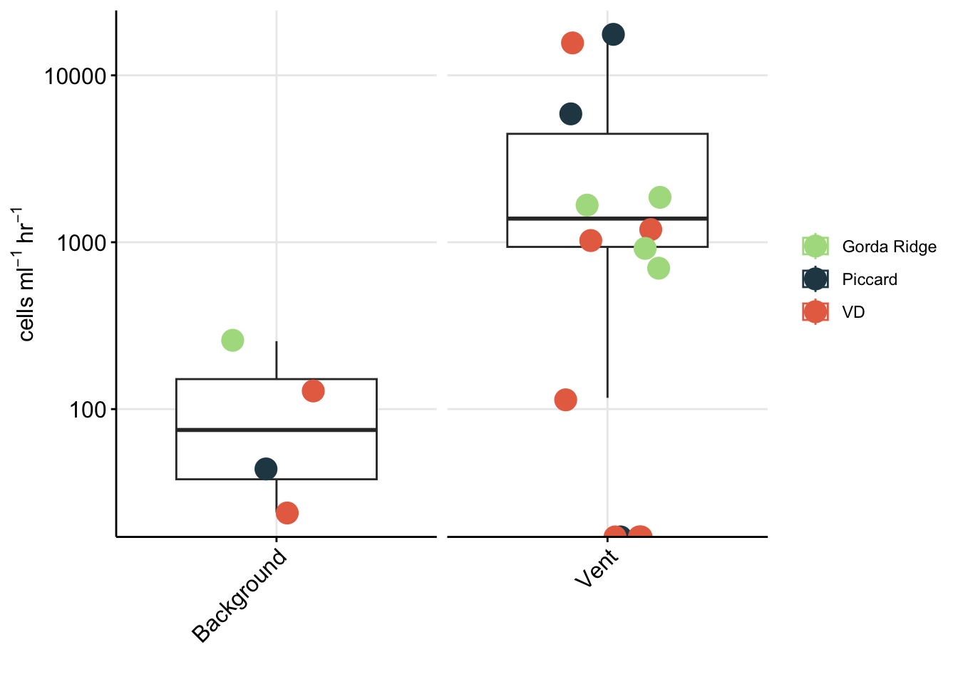

Figure S8

Code

# allrates
# svg("../../../Manuscripts_presentations_reviews/MCR-grazing-2023/svg-files-figures/figS7.svg", h = 4, w = 6)
allrates + scale_y_log10()

Warning: Transformation introduced infinite values in continuous y-axis
Transformation introduced infinite values in continuous y-axis
Transformation introduced infinite values in continuous y-axis
Transformation introduced infinite values in continuous y-axis

Warning: Removed 1 rows containing missing values (`geom_point()`).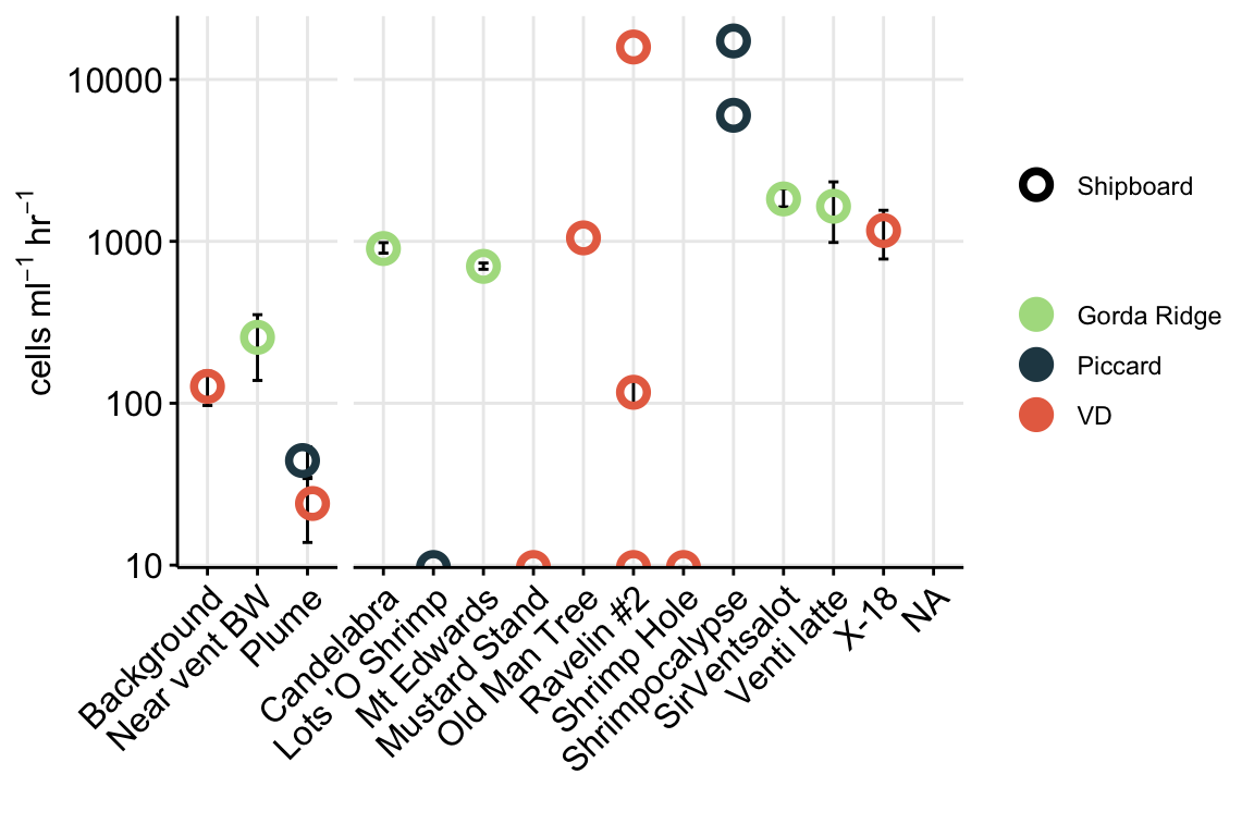

Code

# dev.off()
# allrates + scale_y_continuous(limits = c(0,1000))

Code

# allrates
# svg("../../../Manuscripts_presentations_reviews/MCR-grazing-2023/svg-files-figures/figS7.svg", h = 4, w = 6)
allrates + scale_y_continuous(limits = c(0, 8000))

Warning: Removed 3 rows containing missing values (`geom_point()`).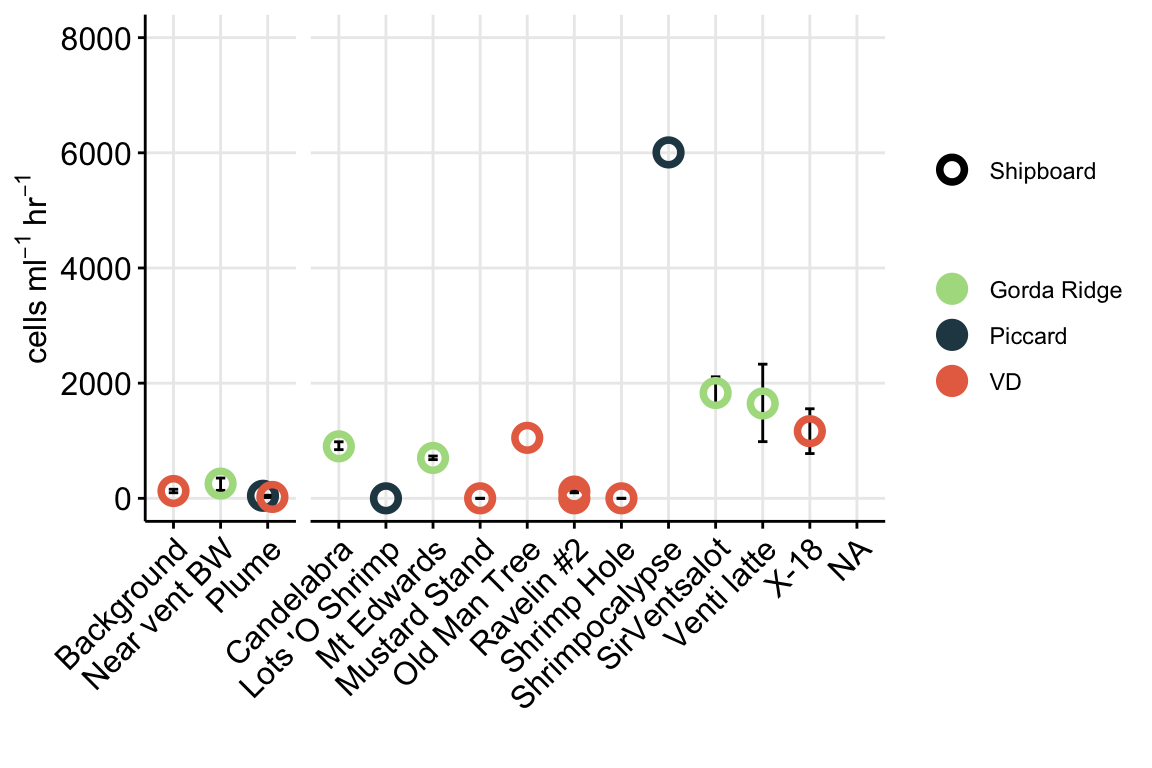

Code

# dev.off()
# allrates + scale_y_continuous(limits = c(0,1000))

Code

# head(all_vents)
all_vents %>% 
  mutate(EXPERIMENTTYPE = case_when(
    EXP == "IGT" ~ "IGT",
    TRUE ~ "Shipboard"
  )) %>% 
  select(EXPERIMENTTYPE, FIELD, NAME, SAMPLE, EXP, SAMPLE_TYPE, starts_with("GRAZING_EFFECT_")) %>% 
  distinct() %>% 
  # filter(SAMPLE_TYPE == "Vent" ) %>% 
    ggplot(aes(y = GRAZING_EFFECT_hr, x = SAMPLE_TYPE)) +
    geom_boxplot() +
    # geom_errorbar(aes(ymax = (GRAZING_EFFECT_hr_max), ymin = (GRAZING_EFFECT_hr_min)), 
                  # width = 0.2, position = position_dodge(width = 0.4), color = "black") +
    geom_jitter(stat = "identity", aes(color = FIELD),
               size = 3, stroke = 2, position = position_dodge(width = 0.4)) +
    scale_shape_manual(values = c(1, 19)) +
    scale_color_manual(values = c("#addd8e", "#264653", "#E76F51")) +
    facet_grid(. ~ SAMPLE_TYPE, scales = "free", space = "free") +
    theme_minimal() +
    theme(panel.grid.major = element_line(), panel.grid.minor = element_blank(),
          panel.background = element_blank(), 
          axis.line = element_line(colour = "black"), 
          axis.text.x = element_text(color="black", size = 12, 
                                     angle = 45, hjust = 1, vjust = 1), 
          axis.text.y = element_text(color="black", size = 12),
          axis.title =element_text(color="black", size = 12),
          axis.ticks = element_line(),
          legend.title = element_blank(),
          strip.placement = "outside",
          strip.text.y = element_text(color="black", size = 12),
          strip.text.x = element_blank())+
    guides(fill = guide_legend(override.aes = list(shape = c(21))),
           shape = guide_legend(override.aes = list(fill = "black"))) +
    labs(x = "", y = bquote("cells"~ml^-1~hr^-1))

Warning: Removed 1 rows containing non-finite values (`stat_boxplot()`).

Warning: Removed 1 rows containing missing values (`geom_point()`).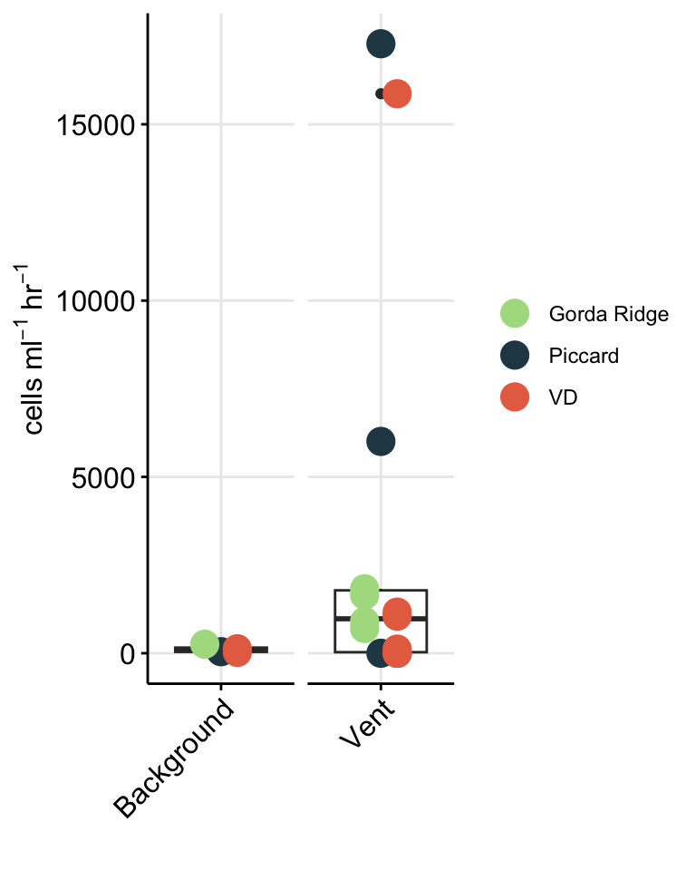

Code

#
 # scale_fill_manual(values = c("#E76F51", "#264653")) +
  # scale_color_manual(values = c("#E76F51", "#264653")) +

Remove undetected grazing rate

Repeat grazing rate plot, but removed undetectable

Code

# unique(all_vents$GRAZING_EFFECT_hr)
allrates_nonzero <- all_vents %>% 
  filter(GRAZING_EFFECT_hr > 0) %>% 
  select(FIELD, NAME, SAMPLE, EXP, SAMPLE_TYPE, starts_with("GRAZING_EFFECT_")) %>% 
  distinct() %>% 
    ggplot(aes(y = GRAZING_EFFECT_hr, x = NAME, fill = FIELD, shape = SAMPLE_TYPE)) +
    geom_errorbar(aes(ymax = (GRAZING_EFFECT_hr_max), ymin = (GRAZING_EFFECT_hr_min)), 
                  width = 0.2, position = position_dodge(width = 0.4)) +
    geom_point(stat = "identity", aes(fill = FIELD, shape = SAMPLE_TYPE),
               color = "black", size = 3, position = position_dodge(width = 0.4)) +
    scale_shape_manual(values = c(21, 24)) +
    scale_fill_manual(values = c("#de2d26", "#1c9099", "#addd8e")) +
    facet_grid(. ~ SAMPLE_TYPE, scales = "free", space = "free") +
    theme_minimal() +
    theme(panel.grid.major = element_line(), panel.grid.minor = element_blank(),
          panel.background = element_blank(), 
          axis.line = element_line(colour = "black"), 
          axis.text.x = element_text(color="black", size = 11, 
                                     angle = 45, hjust = 1, vjust = 1), 
          axis.text.y = element_text(color="black", size = 11),
          axis.title =element_text(color="black", size = 11),
          axis.ticks = element_line(),
          legend.title = element_blank(),
          strip.placement = "outside",
          strip.text.y = element_text(color="black", size = 11),
          strip.text.x = element_blank())+
    guides(fill = guide_legend(override.aes = list(shape = c(21))),
           shape = guide_legend(override.aes = list(fill = "black"))) +
    labs(x = "", y = bquote("cells"~ml^-1~hr^-1))

Code

# svg("compare-all-rates-color-nonZero.svg", h = 4, w = 7)
allrates_nonzero + scale_y_log10()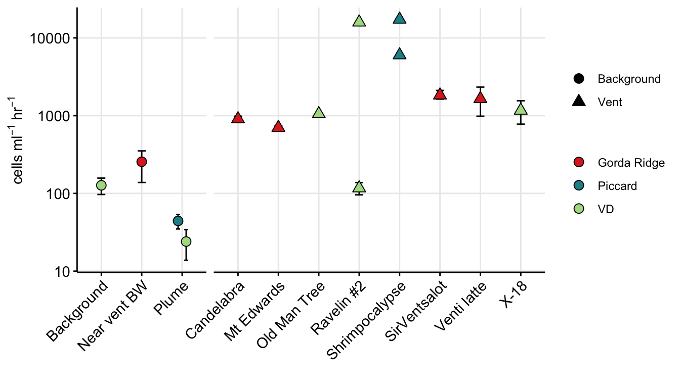

Code

# dev.off()

14.3 Plot variables as a factor of grazing rate.

Figure S7

Code

# svg("../../../Manuscripts_presentations_reviews/MCR-grazing-2023/svg-files-figures/figS6.svg", h = 8, w = 10)
grazing_wenv %>% 
    mutate(TEMP = as.numeric(temp)) %>% 
    mutate(EXP_TYPE = case_when(
      grepl("IGT", Experiment_rep) ~ "IGT",
      TRUE ~ "Shipboard"
    )) %>% 
  unite(SITE_TYPE, SiteOrder, EXP_TYPE, sep = "-", remove = FALSE) %>% 
  filter(!(SITE_TYPE == "NA-IGT")) %>% 
  mutate(EUK_ml = as.character(EUK_ml)) %>% 
  mutate(PROK_ml = as.character(PROK_ml)) %>%
  mutate(temp = as.character(temp),
         pH = as.character(pH),
         mg = as.character(mg),
         h2 = as.character(h2),
         ch4 = as.character(ch4),
         percseawater = as.character(percseawater)) %>% 
  select(SITE_TYPE, SiteOrder, EXP_TYPE, Experiment_rep, GRAZING_EFFECT_hr, EUK_ml, PROK_ml, temp, DEPTH, pH, percseawater, mg, h2, ch4) %>% 
  pivot_longer(cols = EUK_ml:ch4, values_to = "VALUES", values_ptypes = list(VALUES = character())) %>% 
  mutate(VALUES = as.numeric(VALUES)) %>% 
  drop_na() %>% 
  ggplot(aes(x = GRAZING_EFFECT_hr, y = VALUES, 
             color = SITE_TYPE, fill = SITE_TYPE, shape = SITE_TYPE)) +
  geom_point(aes(shape = SITE_TYPE), size = 4, stroke = 2) +
  facet_wrap(~ name, scales = "free") +
  scale_y_continuous() +
  scale_x_log10() +
  scale_shape_manual(values = c(21, 21, 21, 21)) +
  scale_fill_manual(values = c("white", "#264653", "white", "#E76F51")) +
  scale_color_manual(values = c("#264653", "#264653", "#E76F51", "#E76F51")) +
  theme_minimal() +
    theme(panel.grid.minor = element_blank(),
           axis.line = element_line(colour = "black"), 
           axis.text.x = element_text(color="black", size = 13), 
           axis.text.y = element_text(color="black", size = 13),
           axis.title = element_text(color="black", size = 13),
           axis.ticks = element_line(),
           strip.text = element_text(color="black", size = 13), legend.title = element_blank()) +
  labs(x = bquote("Cells consumed "~mL^-1 ~hr^-1), y = bquote("Eukaryote cells "~mL^-1),
       title = "")

Warning: Transformation introduced infinite values in continuous x-axis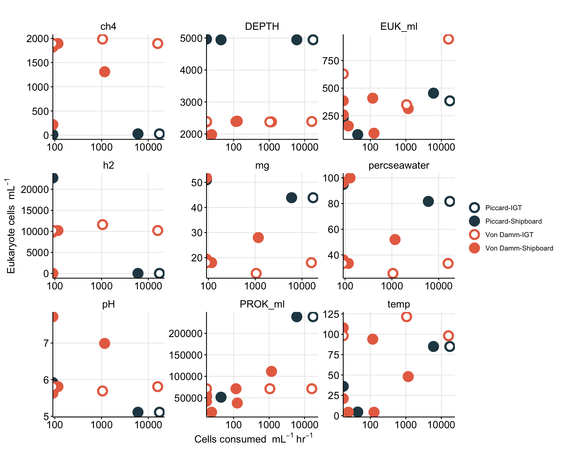

Code

# dev.off()

Code

grazing_wenv_forLM <- grazing_wenv %>% 
  # filter(!(Name == "Shrimpocalypse" & grepl("IGT", Experiment_rep))) %>%
  filter(GRAZING_EFFECT_hr > 0) %>%
    mutate(TEMP = as.numeric(temp)) %>% 
    mutate(EXP_TYPE = case_when(
      grepl("IGT", Experiment_rep) ~ "IGT",
      TRUE ~ "Shipboard"
    )) %>% 
  unite(SITE_TYPE, SiteOrder, EXP_TYPE, sep = "-", remove = FALSE) %>% 
  filter(!(SITE_TYPE == "NA-IGT")) %>% 
  mutate(EUK_ml = as.character(EUK_ml)) %>% 
  mutate(PROK_ml = as.character(PROK_ml),
         PROK_EUK_RATIO = as.character(as.numeric(PROK_ml)/as.numeric(EUK_ml))) %>%
  mutate(temp = as.character(temp),
         pH = as.character(pH),
         mg = as.character(mg),
         h2 = as.character(h2),
         ch4 = as.character(ch4),
         percseawater = as.character(percseawater)) %>% 
  select(SITE_TYPE, SiteOrder, EXP_TYPE, Experiment_rep, GRAZING_EFFECT_hr, CLEARANCE_RATE_ml, SPEC_GRAZE_RATE_hr, BAC_TURNOVER_PERC, EUK_ml, PROK_ml, PROK_EUK_RATIO, temp, DEPTH, pH, percseawater, mg, h2, ch4) %>% 
  pivot_longer(cols = c(GRAZING_EFFECT_hr, CLEARANCE_RATE_ml, SPEC_GRAZE_RATE_hr, BAC_TURNOVER_PERC), names_to = "RATE", values_to = "RATE_VALUE") %>%
  pivot_longer(cols = c(PROK_ml, EUK_ml, temp, DEPTH, pH, percseawater, mg, h2, ch4, PROK_EUK_RATIO), names_to = "PARAMS", values_to = "PARAMS_VALUE") %>%
  data.frame

Code

library(broom)
regression_tmp <- grazing_wenv_forLM %>%
  mutate(PARAMS_VALUE = as.numeric(PARAMS_VALUE)) %>% 
  # Set up the linear regression
  group_by(RATE, PARAMS) %>%
  nest(data = c(-RATE, -PARAMS)) %>%
  mutate(lm_fit = map(data, ~lm(RATE_VALUE ~ PARAMS_VALUE, data = .)),
    tidied = map(lm_fit, tidy)) %>%
  unnest(tidied) %>%
  select(RATE, PARAMS,
    term, estimate) %>%
  pivot_wider(names_from = term, values_from = estimate) %>%
  select(everything(), SLOPE = PARAMS_VALUE) %>%
  data.frame

regression_results_S8 <- grazing_wenv_forLM %>%
  group_by(RATE, PARAMS) %>%
  nest(data = c(-RATE, -PARAMS)) %>%
  mutate(lm_fit = map(data, ~lm(RATE_VALUE ~ PARAMS_VALUE, data = .)),
    glanced = map(lm_fit, glance)) %>%
  unnest(glanced) %>%
  select(RATE, PARAMS, r.squared, adj.r.squared) %>%
  right_join(grazing_wenv_forLM) %>%
  right_join(regression_tmp) %>%
  data.frame

Joining with `by = join_by(RATE, PARAMS)`
Joining with `by = join_by(RATE, PARAMS)`

Supplementary Table

Code

regression_results_TABLE <- regression_results_S8 %>% 
  select(RATE, PARAMS, r.squared, adj.r.squared, SLOPE) %>% 
  distinct()
# write.csv(regression_results_TABLE, file = "output-data/LM-results-table.csv")

Code

# svg("../../../Manuscripts_presentations_reviews/MCR-grazing-2023/svg-files-figures/figS6.svg", h = 8, w = 10)
grazing_for_supp <- regression_results_S8

# y = mx+b
# 0 = slope (x) + b
# solve for b
plot_r2 <- grazing_for_supp %>% 
  ggplot(aes(x = as.numeric(RATE_VALUE), y = as.numeric(PARAMS_VALUE), 
             color = SITE_TYPE, fill = SITE_TYPE, shape = SITE_TYPE)) +
  geom_point(aes(shape = SITE_TYPE), size = 4, stroke = 2) +
  facet_wrap(~ PARAMS + round(r.squared, 3), scales = "free", ncol = 5,
             labeller = label_parsed) +
  scale_y_continuous() +
  scale_x_log10(labels = scientific_10) +
  scale_shape_manual(values = c(21, 21, 21, 21)) +
  scale_fill_manual(values = c("white", "#264653", "white", "#E76F51")) +
  scale_color_manual(values = c("#264653", "#264653", "#E76F51", "#E76F51")) +
  theme_minimal() +
    theme(panel.grid.minor = element_blank(),
           axis.line = element_line(colour = "black"), 
           axis.text.x = element_text(color="black", size = 13), 
           axis.text.y = element_text(color="black", size = 13),
           axis.title = element_text(color="black", size = 13),
           axis.ticks = element_line(),
           strip.text = element_text(color="black", size = 13), legend.title = element_blank()) +
  labs(x = bquote("Cells consumed "~mL^-1 ~hr^-1), y = bquote("Eukaryote cells "~mL^-1),
       title = "")

plot_wslope <- grazing_for_supp %>% 
    mutate(b = (SLOPE)*(`X.Intercept.`)) %>% 
  mutate(new_xint = ((0 - b)/SLOPE)) %>% 
    mutate(new_xint_2 = case_when(
      `X.Intercept.` < 0 ~ (`X.Intercept.`)*(-1),
      `X.Intercept.` > 0 ~ (`X.Intercept.`),
    )) %>% 
  filter(!is.na(PARAMS_VALUE)) %>% 
  ggplot(aes(x = as.numeric(RATE_VALUE), y = as.numeric(PARAMS_VALUE), 
             color = SITE_TYPE, fill = SITE_TYPE, shape = SITE_TYPE)) +
  geom_point(aes(shape = SITE_TYPE), size = 4, stroke = 2) +
  facet_wrap(~ PARAMS + round(r.squared, 3), scales = "free", ncol = 5,
             labeller = label_parsed) +
  # scale_y_continuous() +
  # scale_x_log10() +
  scale_x_continuous(trans=log10_trans(),
                       breaks = trans_breaks("log10", function(x) 10^x),
                       labels = trans_format("log10", math_format(10^.x))) +
    geom_abline(aes(slope = (SLOPE), intercept = (`X.Intercept.`)), color = "black", linetype = "dashed", size = 0.5) +
  # geom_abline(aes(slope = (SLOPE), yintercept = (b)), color = "black", linetype = "dashed", size = 0.5) +
  scale_shape_manual(values = c(21, 21, 21, 21)) +
  scale_fill_manual(values = c("white", "#264653", "white", "#E76F51")) +
  scale_color_manual(values = c("#264653", "#264653", "#E76F51", "#E76F51")) +
  theme_minimal() +
    theme(panel.grid.minor = element_blank(),
           axis.line = element_line(colour = "black"), 
           axis.text.x = element_text(color="black", size = 13), 
           axis.text.y = element_text(color="black", size = 13),
           axis.title = element_text(color="black", size = 13),
           axis.ticks = element_line(),
           strip.text = element_text(color="black", size = 13), legend.title = element_blank()) +
  labs(x = bquote("Cells consumed "~mL^-1 ~hr^-1), y = bquote("Eukaryote cells "~mL^-1),
       title = "")

# plot_wslope

Figure S7 #2

Supplementary figure

Code

# svg("../../../Manuscripts_presentations_reviews/MCR-grazing-2023/svg-files-figures/figS7_log.svg", h = 8, w = 16)

# plot_r2

# svg("../../../Manuscripts_presentations_reviews/MCR-grazing-2023/svg-files-figures/figS7_slope.svg", h = 8, w = 16)
# 
# plot_wslope

# dev.off()

15 Linear regression & tidy models

Use tidymodels to perform linear regression.

15.1 MCR and GR data as input

Code

library(broom)
# ?pivot_longer
# e IGT
# head(all_vents)
# regression_input <- all_vents %>%
#   # filter(!(SAMPLE == "Piccard-Shrimpocalypse" & EXP == "IGT")) %>%
#   filter(!is.na(Highest.Temp)) %>%
#     select(FIELD, NAME, SAMPLE, SAMPLE_TYPE, EXP, PROK_ml, EUK_ml, GRAZING_EFFECT_hr, BAC_TURNOVER_PERC, TEMP = Highest.Temp) %>%
#   mutate(PROK_EUK_RATIO = (PROK_ml/EUK_ml)) %>%
#   pivot_longer(cols = c(GRAZING_EFFECT_hr, BAC_TURNOVER_PERC), names_to = "RATE", values_to = "RATE_VALUE") %>%
#   pivot_longer(cols = c(PROK_ml, EUK_ml, PROK_EUK_RATIO, TEMP), names_to = "PARAMS", values_to = "PARAMS_VALUE") %>%
#   data.frame
# 
# regression_tmp <- regression_input %>%
#   # Set up the linear regression
#   group_by(RATE, PARAMS) %>%
#   nest(-RATE, -PARAMS) %>%
#   mutate(lm_fit = map(data, ~lm(RATE_VALUE ~ PARAMS_VALUE, data = .)),
#     tidied = map(lm_fit, tidy)) %>%
#   unnest(tidied) %>%
#   select(RATE, PARAMS,
#     term, estimate) %>%
#   pivot_wider(names_from = term, values_from = estimate) %>%
#   select(everything(), SLOPE = PARAMS_VALUE) %>%
#   data.frame
# 
# regression_results <- regression_input %>%
#   group_by(RATE, PARAMS) %>%
#   nest(-RATE, -PARAMS) %>%
#   mutate(lm_fit = map(data, ~lm(RATE_VALUE ~ PARAMS_VALUE, data = .)),
#     glanced = map(lm_fit, glance)) %>%
#   unnest(glanced) %>%
#   select(RATE, PARAMS, r.squared, adj.r.squared) %>%
#   right_join(regression_tmp) %>%
#   right_join(regression_input) %>%
#   data.frame

# View(regression_results)

Plot results from regression

Code

# regression_results %>%
#   # filter(RATE == "GRAZING_EFFECT_hr") %>%
#   # filter(PARAMS == "TEMP") %>%
#   ggplot(aes(x = PARAMS_VALUE, y = RATE_VALUE, shape = SAMPLE_TYPE, fill = FIELD)) +
#     geom_abline(aes(slope = SLOPE, intercept = `X.Intercept.`), color = "black", linetype = "dashed", size = 0.5) +
#     geom_point(color = "black", aes(shape = SAMPLE_TYPE, fill = FIELD)) +
#     scale_shape_manual(values = c(21, 24)) +
#     scale_fill_manual(values = c("#476AA7","#7299CE", "#A2937A")) +
#     facet_wrap(PARAMS ~ RATE + round(r.squared, 3), scales = "free", ncol = 5,
#              strip.position = "bottom", labeller = label_parsed) +
#   theme_bw() +
#   theme(
#     strip.background = element_blank(),
#     strip.placement = "outside",
#     strip.text = element_text(color = "black", size = 10),
#     axis.title = element_text(color = "black", size = 10),
#     legend.title = element_blank()) # +
# labs(y = bquote("Cells "~mL^-1 ~hr^-1), x = "Temperature (C)")

15.2 MCR only

repeat MCR only

Code

library(broom)
# ?pivot_longer
# unique(all_vents$FIELD)
regression_input <- all_vents %>% 
  filter(!(FIELD == "Gorda Ridge")) %>% 
  # filter(!(SAMPLE == "Piccard-Shrimpocalypse" & EXP == "IGT")) %>% 
  filter(!is.na(Highest.Temp)) %>% 
    select(FIELD, NAME, SAMPLE, SAMPLE_TYPE, EXP, PROK_ml, EUK_ml, GRAZING_EFFECT_hr, BAC_TURNOVER_PERC, TEMP = Highest.Temp) %>% 
  mutate(PROK_EUK_RATIO = (PROK_ml/EUK_ml)) %>% 
  pivot_longer(cols = c(GRAZING_EFFECT_hr, BAC_TURNOVER_PERC), names_to = "RATE", values_to = "RATE_VALUE") %>% 
  pivot_longer(cols = c(PROK_ml, EUK_ml, PROK_EUK_RATIO, TEMP), names_to = "PARAMS", values_to = "PARAMS_VALUE") %>% 
  data.frame
head(regression_input)

    FIELD           NAME              SAMPLE SAMPLE_TYPE  EXP              RATE
1 Piccard Lots 'O Shrimp Piccard-LotsOShrimp        Vent LV24 GRAZING_EFFECT_hr
2 Piccard Lots 'O Shrimp Piccard-LotsOShrimp        Vent LV24 GRAZING_EFFECT_hr
3 Piccard Lots 'O Shrimp Piccard-LotsOShrimp        Vent LV24 GRAZING_EFFECT_hr
4 Piccard Lots 'O Shrimp Piccard-LotsOShrimp        Vent LV24 GRAZING_EFFECT_hr
5 Piccard Lots 'O Shrimp Piccard-LotsOShrimp        Vent LV24 BAC_TURNOVER_PERC
6 Piccard Lots 'O Shrimp Piccard-LotsOShrimp        Vent LV24 BAC_TURNOVER_PERC
  RATE_VALUE         PARAMS PARAMS_VALUE
1          0        PROK_ml    53878.000
2          0         EUK_ml      230.910
3          0 PROK_EUK_RATIO      233.329
4          0           TEMP       36.000
5          0        PROK_ml    53878.000
6          0         EUK_ml      230.910

Code

regression_tmp <- regression_input %>% 
  # Set up the linear regression
  group_by(RATE, PARAMS) %>% 
  nest(-RATE, -PARAMS) %>% 
  mutate(lm_fit = map(data, ~lm(RATE_VALUE ~ PARAMS_VALUE, data = .)), 
    tidied = map(lm_fit, tidy)) %>% 
  unnest(tidied) %>% 
  select(RATE, PARAMS, 
    term, estimate) %>% 
  pivot_wider(names_from = term, values_from = estimate) %>% 
  select(everything(), SLOPE = PARAMS_VALUE) %>%
  data.frame

Warning: Supplying `...` without names was deprecated in tidyr 1.0.0.
ℹ Please specify a name for each selection.
ℹ Did you want `data = c(-RATE, -PARAMS)`?

Code

regression_results_mcr <- regression_input %>% 
  group_by(RATE, PARAMS) %>% 
  nest(-RATE, -PARAMS) %>% 
  mutate(lm_fit = map(data, ~lm(RATE_VALUE ~ PARAMS_VALUE, data = .)),
    glanced = map(lm_fit, glance)) %>% 
  unnest(glanced) %>% 
  select(RATE, PARAMS, r.squared, adj.r.squared) %>% 
  right_join(regression_tmp) %>%
  right_join(regression_input) %>%
  data.frame

Warning: Supplying `...` without names was deprecated in tidyr 1.0.0.
ℹ Please specify a name for each selection.
ℹ Did you want `data = c(-RATE, -PARAMS)`?

Joining with `by = join_by(RATE, PARAMS)`
Joining with `by = join_by(RATE, PARAMS)`

Code

# View(regression_results_mcr)

Plot results from regression

Code

regression_results_mcr %>% 
  # filter(RATE == "GRAZING_EFFECT_hr") %>%
  # filter(PARAMS == "TEMP") %>% 
  ggplot(aes(x = PARAMS_VALUE, y = RATE_VALUE, shape = SAMPLE_TYPE, fill = FIELD)) +
    geom_abline(aes(slope = SLOPE, intercept = `X.Intercept.`), color = "black", linetype = "dashed", size = 0.5) +
    geom_point(color = "black", aes(shape = SAMPLE_TYPE, fill = FIELD)) +
    scale_shape_manual(values = c(21, 24)) +
    scale_fill_manual(values = c("#476AA7","#7299CE", "#A2937A")) +
    facet_wrap(PARAMS ~ RATE + round(r.squared, 3), scales = "free", ncol = 5,
             strip.position = "bottom", labeller = label_parsed) +
  theme_bw() +
  theme(
    strip.background = element_blank(),
    strip.placement = "outside",
    strip.text = element_text(color = "black", size = 10),
    axis.title = element_text(color = "black", size = 10),
    legend.title = element_blank()) # +

Code

  # labs(y = bquote("Cells "~mL^-1 ~hr^-1), x = "Temperature (C)")

15.3 MCR vent sites only

Repeat with only vent sites & remove undetected grazing.

Code

# head(all_vents)
# range(all_vents$GRAZING_EFFECT_hr)

Code

library(broom)
# ?pivot_longer
# unique(all_vents$FIELD)
regression_input <- all_vents %>% 
  filter(!(FIELD == "Gorda Ridge")) %>% 
  filter(!(NAME == "Background")) %>% filter(!(NAME == "Plume")) %>% 
  filter(GRAZING_EFFECT_hr > 0) %>% 
  # filter(!(SAMPLE == "Piccard-Shrimpocalypse" & EXP == "IGT")) %>% 
  filter(!is.na(Highest.Temp)) %>% 
    select(FIELD, NAME, SAMPLE, SAMPLE_TYPE, EXP, PROK_ml, EUK_ml, GRAZING_EFFECT_hr, BAC_TURNOVER_PERC, TEMP = Highest.Temp) %>% 
  mutate(PROK_EUK_RATIO = (PROK_ml/EUK_ml)) %>% 
  pivot_longer(cols = c(GRAZING_EFFECT_hr, BAC_TURNOVER_PERC), names_to = "RATE", values_to = "RATE_VALUE") %>% 
  pivot_longer(cols = c(PROK_ml, EUK_ml, PROK_EUK_RATIO, TEMP), names_to = "PARAMS", values_to = "PARAMS_VALUE") %>% 
  data.frame

regression_tmp <- regression_input %>% 
  # Set up the linear regression
  group_by(RATE, PARAMS) %>% 
  nest(-RATE, -PARAMS) %>% 
  mutate(lm_fit = map(data, ~lm(RATE_VALUE ~ PARAMS_VALUE, data = .)), 
    tidied = map(lm_fit, tidy)) %>% 
  unnest(tidied) %>% 
  select(RATE, PARAMS, 
    term, estimate) %>% 
  pivot_wider(names_from = term, values_from = estimate) %>% 
  select(everything(), SLOPE = PARAMS_VALUE) %>%
  data.frame

Warning: Supplying `...` without names was deprecated in tidyr 1.0.0.
ℹ Please specify a name for each selection.
ℹ Did you want `data = c(-RATE, -PARAMS)`?

Code

regression_results_vent <- regression_input %>% 
  group_by(RATE, PARAMS) %>% 
  nest(-RATE, -PARAMS) %>% 
  mutate(lm_fit = map(data, ~lm(RATE_VALUE ~ PARAMS_VALUE, data = .)),
    glanced = map(lm_fit, glance)) %>% 
  unnest(glanced) %>% 
  select(RATE, PARAMS, r.squared, adj.r.squared) %>% 
  right_join(regression_tmp) %>%
  right_join(regression_input) %>%
  data.frame

Warning: Supplying `...` without names was deprecated in tidyr 1.0.0.
ℹ Please specify a name for each selection.
ℹ Did you want `data = c(-RATE, -PARAMS)`?

Joining with `by = join_by(RATE, PARAMS)`
Joining with `by = join_by(RATE, PARAMS)`

Code

# View(regression_results_vent)

Plot results from regression

Code

regression_results_vent %>% 
  # filter(RATE == "GRAZING_EFFECT_hr") %>%
  # filter(PARAMS == "TEMP") %>% 
  ggplot(aes(x = PARAMS_VALUE, y = RATE_VALUE, shape = SAMPLE_TYPE, fill = FIELD)) +
    geom_abline(aes(slope = SLOPE, intercept = `X.Intercept.`), color = "black", linetype = "dashed", size = 0.5) +
    geom_point(color = "black", aes(shape = SAMPLE_TYPE, fill = FIELD)) +
    scale_shape_manual(values = c(21, 24)) +
    scale_fill_manual(values = c("#476AA7","#7299CE", "#A2937A")) +
    facet_wrap(PARAMS ~ RATE + round(r.squared, 3), scales = "free", ncol = 5,
             strip.position = "bottom", labeller = label_parsed) +
  theme_bw() +
  theme(
    strip.background = element_blank(),
    strip.placement = "outside",
    strip.text = element_text(color = "black", size = 10),
    axis.title = element_text(color = "black", size = 10),
    legend.title = element_blank()) # +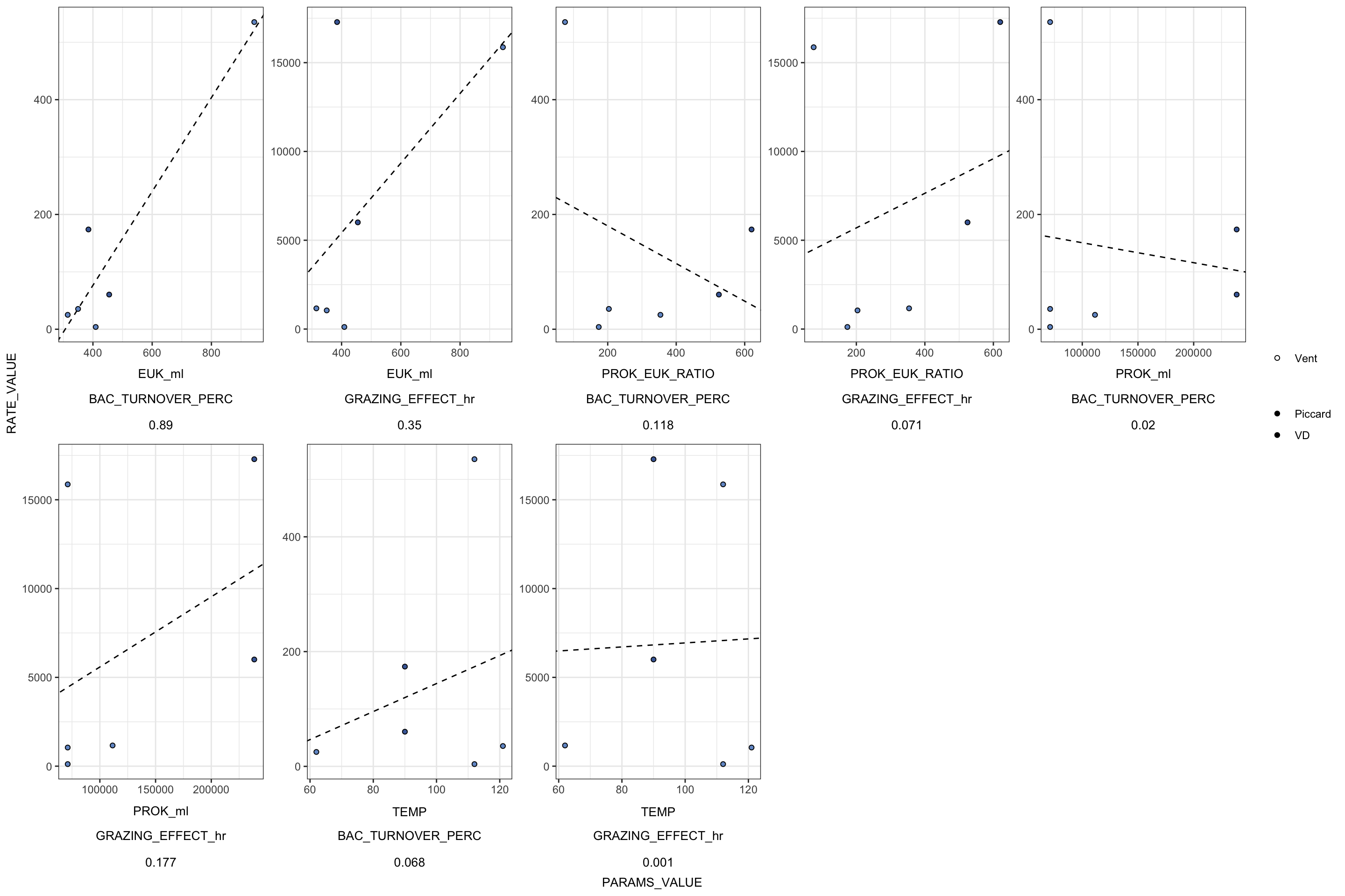

Code

  # labs(y = bquote("Cells "~mL^-1 ~hr^-1), x = "Temperature (C)")

Regression thoughts: Unremarkable r squared values (numbers at the bottom of each plot). Some trends, mainly associated with temperature.

Bacterial abundance typically increases with temperature (White et al. 1991) - which could ultimately increase bacterial ingestion rate and total protist cells. But at this type of niche environment, I hypothesize that there is a trend but threshold of not detected grazing under certain conditions.

If euk per ml numbers are high, but we see lower grazing rates, could this be competition? Curds and Cockburn 1968. Additionally with temperature… in Vaque et al GRF (specific grazing rates of flagellates) increased with temperature, but overall grazing rate reached a plateau at 18C. Does this mean that temperature will be an important factor depending on the community diversity?

Code

head(all_vents)

    FIELD           NAME                 SAMPLE          EXP PROK_ml  EUK_ml
1 Piccard Lots 'O Shrimp    Piccard-LotsOShrimp         LV24   53878 230.910
2 Piccard Lots 'O Shrimp    Piccard-LotsOShrimp         LV24   53878 230.910
3 Piccard          Plume          Piccard-Plume    Niskin 10   51429  79.301
4 Piccard Shrimpocalypse Piccard-Shrimpocalypse         LV13  238590 454.820
5      VD     Background                 VD-BSW Niskins 8-10   37890  91.838
6      VD     Background                 VD-BSW Niskins 8-10   37890  91.838
  GRAZING_EFFECT_hr GRAZING_EFFECT_hr_min GRAZING_EFFECT_hr_max
1            0.0000                    NA                    NA
2            0.0000                    NA                    NA
3           44.2591              34.87211              53.64608
4         6006.9122                    NA                    NA
5          127.0655              96.81191             157.31912
6          127.0655              96.81191             157.31912
  BAC_TURNOVER_PERC Highest.Temp pH Mg H2S H2 CH4 SAMPLE_TYPE
1          0.000000       36.000 NA NA  NA NA  NA        Vent
2          0.000000       35.000 NA NA  NA NA  NA        Vent
3          2.065407        4.722 NA NA  NA NA  NA  Background
4         60.424114       90.000 NA NA  NA NA  NA        Vent
5          8.048489        4.181 NA NA  NA NA  NA  Background
6          8.048489        4.100 NA NA  NA NA  NA  Background

Code

allvent_data <- all_vents %>% 
  mutate(PROK_EUK_RATIO = (PROK_ml/EUK_ml))
# head(allvent_data)

Function to plot results by two parameters.

Code

two_params <- function(df, x_var, y_var, x_title, y_title){
  X_VAR <- enquo(x_var)
  Y_VAR <- enquo(y_var)
  df %>% 
  select(FIELD, NAME, SAMPLE, EXP, X = !!X_VAR, Y = !!Y_VAR) %>% 
  distinct() %>% 
  ggplot(aes(x = X, y = Y)) +
    geom_point(size = 3, shape = 21, color = "black", aes(fill = FIELD)) +
    geom_abline(slope = 1, intercept = 0) +
    theme_minimal() +
    labs(x = x_title, y = y_title)
}

15.4 Plot temperature by euk:prok and then euk and prok

Code

two_params(allvent_data, `PROK_EUK_RATIO`, `Highest.Temp`, "Prok:Euk ratio", "Temperature (max)")

Warning: Removed 6 rows containing missing values (`geom_point()`).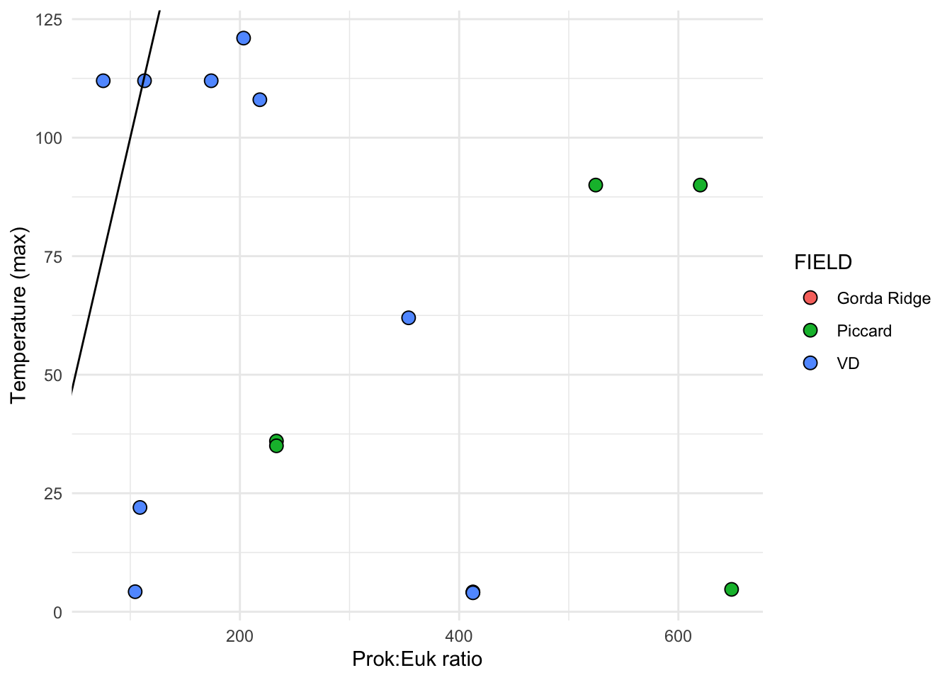

15.5 Plot temperature by grazing rate

Code

names(allvent_data)

 [1] "FIELD"                 "NAME"                  "SAMPLE"               
 [4] "EXP"                   "PROK_ml"               "EUK_ml"               
 [7] "GRAZING_EFFECT_hr"     "GRAZING_EFFECT_hr_min" "GRAZING_EFFECT_hr_max"
[10] "BAC_TURNOVER_PERC"     "Highest.Temp"          "pH"                   
[13] "Mg"                    "H2S"                   "H2"                   
[16] "CH4"                   "SAMPLE_TYPE"           "PROK_EUK_RATIO"       

Code

# two_params(allvent_data, ugC_L_perday, `Highest.Temp`, "ugC_L_perday", "Temperature (max)")
# two_params(allvent_data, ugC_L_perday, EUK_ml, "ugC_L_perday", "Euk cells per ml") + scale_y_log10()

# two_params(allvent_data, EUK_ml, PROK_ml, "Euk", "Prok") + scale_y_log10() + scale_x_log10()

16 Carbon biomass investigation

Code

# head(all_vents)
# GRAZING_EFFECT_hr = "Cells~mL^{-1}~hr^{-1}"

If we assume that carbon content per prey cell is between 86 - 300 fgC per cell. What does the amount consumed look like?

Code

# Create a new data frame
# carbon_density <- crossing(fgC_cell = seq(86, 300, by = 1), 
#                              GRAZING_EFFECT_hr = seq(min(all_vents$GRAZING_EFFECT_hr),
#                                                   max(all_vents$GRAZING_EFFECT_hr),
#                                                   length.out = 215))  %>%
#   mutate(fgC_ml_perday = ((GRAZING_EFFECT_hr*24) * fgC_cell),
#     ugC_L_perday = (fgC_ml_perday * (1e-09) * 1000)
#     ) %>%
#   data.frame
# 
# # unique(all_vents$GRAZING_EFFECT_hr)
# 
# samples_lines <- select(all_vents, GRAZING_EFFECT_hr, FIELD) %>% 
#   distinct() %>% 
#   crossing(fgC_cell = seq(86, 300, by = 20)) %>%
#   mutate(fgC_ml_perday = ((GRAZING_EFFECT_hr*24) * fgC_cell),
#     ugC_L_perday = (fgC_ml_perday * (1e-09) * 1000)
#     )

Code

# ggplot(carbon_density, aes(x = fgC_cell, y = GRAZING_EFFECT_hr)) +
#   geom_raster(aes(fill = ugC_L_perday)) +
#   scale_fill_gradientn(colors = c("#fef0d9", "#b30000"), name = bquote("ug C"~L^-1 ~day^-1)) +
#   # scale_fill_discrete(name = "New Legend Title")
#   scale_y_continuous(expand = c(0,0)) +
#   scale_x_continuous(expand = c(0,0)) +
#   theme_bw() +
#   theme(axis.text = element_text(color = "black"),
#         rect = element_rect(fill = "transparent"),
#         panel.background = element_rect(fill = "transparent"),
#         plot.background = element_rect(fill = "transparent", color = NA)) +
#   labs(y = bquote("Cells "~mL^-1 ~consumed ~hr^-1), x = bquote("fg C"~cell^-1)) +
#   geom_point(data = samples_lines,
#             aes(x = 87,
#             y = GRAZING_EFFECT_hr, shape = FIELD), size = 1)

Eukaryote biomass comparison with measured vs. literature

Code

# Repeated in ASV code right now!
# plot_metadata <- env_params %>% 
#   filter(SAMPLETYPE != "Incubation") %>%
#   filter(VENT != "Quakeplume") %>% 
#   select(SITE, VENT, SAMPLETYPE, TEMP, DEPTH, starts_with("PROK_"), starts_with("EUK_"), starts_with("GRAZING_EFFECT_hr"))

Code

# head(plot_metadata)
# plot_metadata %>% 
#   filter(!is.na(Euk_biomass_Hu)) %>% 
#   mutate(Euk_biomass_Hu_fg = Euk_biomass_Hu * 1000000000,
#          Euk_biomass_lit_fg = Euk_biomass_lit * 1000000000) %>% 
#   ggplot(aes(y = VENT)) +
#   geom_point(aes(x = Euk_biomass_Hu_fg), color = "black", fill = "darkgreen", shape = 21, size = 4) +
#   geom_point(aes(x = Euk_biomass_lit), color = "black", fill = "lightgreen", shape = 21, size = 4) +
#   scale_x_log10(labels = function(x) format(x, scientific = TRUE)) +
#   theme_minimal() +
#   theme(axis.text = element_text(color = "black")) +
#   facet_grid(SAMPLETYPE ~ ., space = "free", scales = "free") +
#   labs(x = "fg C of eukaryote population", y = "")

17 Prediction of MCR data with parameters

Best model to estimate community grazing rate in Vaque et al. considered FLP uptake and similar experiments (in contrast to disappearance experiments).

From Vaque et al. 1994 paper equation (1):

See Figure 6

log(GT) = -3.21 + 0.99 log (HNF) + 0.028 (T) + 0.55 log(BAC)

GT = grazing rate (cells ml-1 hr-1) HNF = heterotrophic nanoflagellates (cells ml-1) T = temperature (C) BAC = prokaryote abundance (cells ml-1)

Start with non-zero grazing rate values, etc. Where… GT == Grazing effect hr HNF == Euk_ml BAC == PROK_ml T == highest temp

We only have these for MCR data.. can include GR for the “predicting euk_ml”

Function to use above formula and estimate

Code

est_predicted <- function(df, TITLE){
  df_out <- df %>% 
  select(FIELD, NAME, SAMPLE, EXP, PROK_ml, EUK_ml, GRAZING_EFFECT_hr, Highest.Temp) %>% 
    filter(GRAZING_EFFECT_hr > 0) %>% 
  group_by(FIELD, NAME, SAMPLE, EXP, PROK_ml, EUK_ml, GRAZING_EFFECT_hr) %>% 
  summarise(TEMP = mean(Highest.Temp)) %>% 
  distinct() %>% 
  mutate(PREDICTED_TEMP = (((log10(GRAZING_EFFECT_hr)) + 3.21 - (0.99*log10(EUK_ml)) - (0.55*log10(PROK_ml))) / 0.028),
         PREDICTED_GRAZING_EFFECT_hr = (10^(-3.21 + (0.99*log10(EUK_ml)) + (0.028*TEMP) + (0.55*(log10(PROK_ml))))),
         PREDICTED_EUK = (10^(((log10(GRAZING_EFFECT_hr)) + 3.21 - (0.55*log10(PROK_ml)) - (0.028*TEMP))/0.99)),
         PREDICTED_PROK = (10^(((log10(GRAZING_EFFECT_hr)) + 3.21 - (0.99*log10(EUK_ml)) - (0.028*TEMP))/0.55)))
  # Plots
  df_out %>% 
  ggplot(aes(x = PREDICTED_GRAZING_EFFECT_hr, y = GRAZING_EFFECT_hr)) +
    geom_point(size = 3, color = "black", fill = "red", shape = 21) + theme_bw() + geom_abline(slope = 1, intercept = 0) +
  df_out %>% 
  ggplot(aes(x = log10(PREDICTED_GRAZING_EFFECT_hr), y = log10(GRAZING_EFFECT_hr))) +
    geom_point(size = 3, color = "black", fill = "red", shape = 21) + theme_bw() +  geom_abline(slope = 1, intercept = 0) +
  df_out %>% 
  ggplot(aes(x = PREDICTED_EUK, y = EUK_ml)) +
    geom_point(size = 3, color = "black", fill = "darkgreen", shape = 21) + theme_bw() + geom_abline(slope = 1, intercept = 0) +
  df_out %>% 
  ggplot(aes(x = log10(PREDICTED_EUK), y = log10(EUK_ml))) +
    geom_point(size = 3, color = "black", fill = "darkgreen", shape = 21) + theme_bw() + geom_abline(slope = 1, intercept = 0) +
  df_out %>% 
  ggplot(aes(x = PREDICTED_PROK, y = PROK_ml)) +
    geom_point(size = 3, color = "black", fill = "blue", shape = 21) + theme_bw() + geom_abline(slope = 1, intercept = 0) +
  df_out %>% 
  ggplot(aes(x = log10(PREDICTED_PROK), y = log10(PROK_ml))) +
    geom_point(size = 3, color = "black", fill = "blue", shape = 21) + theme_bw() + geom_abline(slope = 1, intercept = 0) +
  df_out %>% 
  ggplot(aes(x = PREDICTED_TEMP, y = TEMP)) +
    geom_point(size = 3, color = "black", fill = "orange", shape = 21) + theme_bw() + geom_abline(slope = 1, intercept = 0) +
  df_out %>% 
  ggplot(aes(x = log10(PREDICTED_TEMP), y = log10(TEMP))) +
    geom_point(size = 3, color = "black", fill = "orange", shape = 21) + theme_bw() + geom_abline(slope = 1, intercept = 0) +
  patchwork::plot_layout(ncol = 4) + plot_annotation(title = TITLE)
  # return(df_out)
  }
# head(all_vents)
# unique(all_vents$NAME)
# range(all_vents$Highest.Temp)

Code

est_predicted(all_vents, "all values")

`summarise()` has grouped output by 'FIELD', 'NAME', 'SAMPLE', 'EXP',
'PROK_ml', 'EUK_ml'. You can override using the `.groups` argument.

Warning: Removed 5 rows containing missing values (`geom_point()`).
Removed 5 rows containing missing values (`geom_point()`).
Removed 5 rows containing missing values (`geom_point()`).
Removed 5 rows containing missing values (`geom_point()`).
Removed 5 rows containing missing values (`geom_point()`).
Removed 5 rows containing missing values (`geom_point()`).
Removed 5 rows containing missing values (`geom_point()`).
Removed 5 rows containing missing values (`geom_point()`).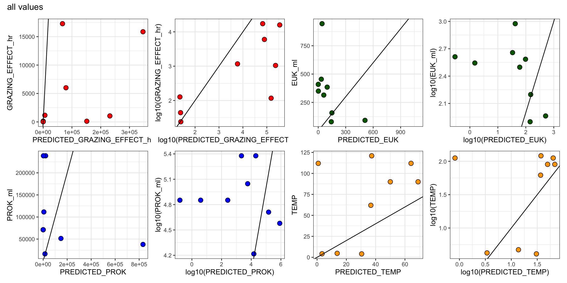

Code

mcr <- c("Von Damm", "Piccard")
bsw <- c("Backgound", "BSW", "Plume", "Near vent BW")

# est_predicted(all_vents %>% filter(FIELD %in% mcr), "Mid-Cayman Rise only")

# est_predicted(all_vents %>% filter(FIELD %in% mcr) %>% filter(GRAZING_EFFECT_hr > 0), "Mid-Cayman Rise only, no undetected")

est_predicted(all_vents %>% filter(FIELD %in% mcr) %>% filter(GRAZING_EFFECT_hr > 0) %>% filter(!(NAME %in% bsw)), "Mid-Cayman Rise only, no undetected, vents only")

`summarise()` has grouped output by 'FIELD', 'NAME', 'SAMPLE', 'EXP',
'PROK_ml', 'EUK_ml'. You can override using the `.groups` argument.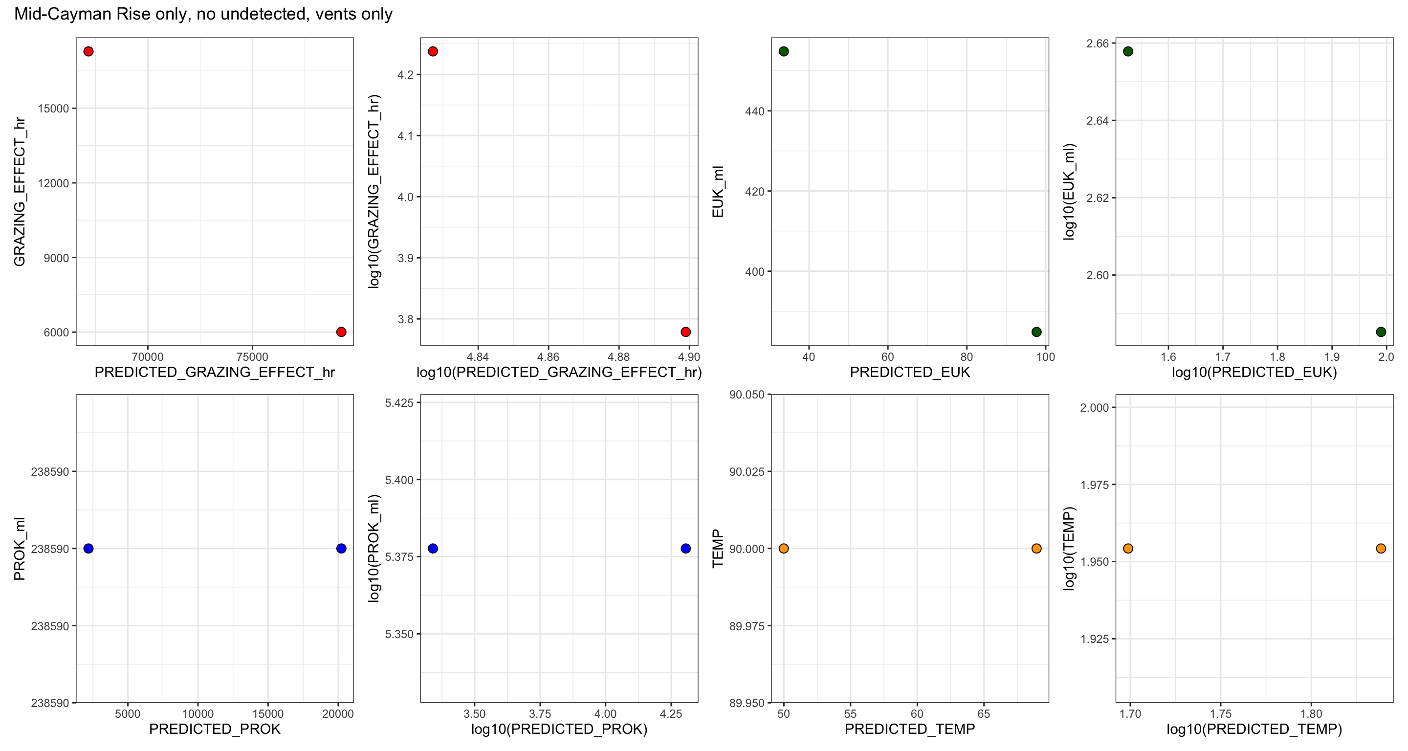

Code

# View(all_vents)
# est_predicted(all_vents %>% filter(!(NAME %in% bsw)), "Vent samples only")

est_predicted(all_vents %>% filter(!(NAME %in% bsw)) %>% filter(GRAZING_EFFECT_hr > 0), "Vent samples only where grazing was detected")

`summarise()` has grouped output by 'FIELD', 'NAME', 'SAMPLE', 'EXP',
'PROK_ml', 'EUK_ml'. You can override using the `.groups` argument.

Warning: Removed 4 rows containing missing values (`geom_point()`).
Removed 4 rows containing missing values (`geom_point()`).
Removed 4 rows containing missing values (`geom_point()`).
Removed 4 rows containing missing values (`geom_point()`).
Removed 4 rows containing missing values (`geom_point()`).
Removed 4 rows containing missing values (`geom_point()`).
Removed 4 rows containing missing values (`geom_point()`).
Removed 4 rows containing missing values (`geom_point()`).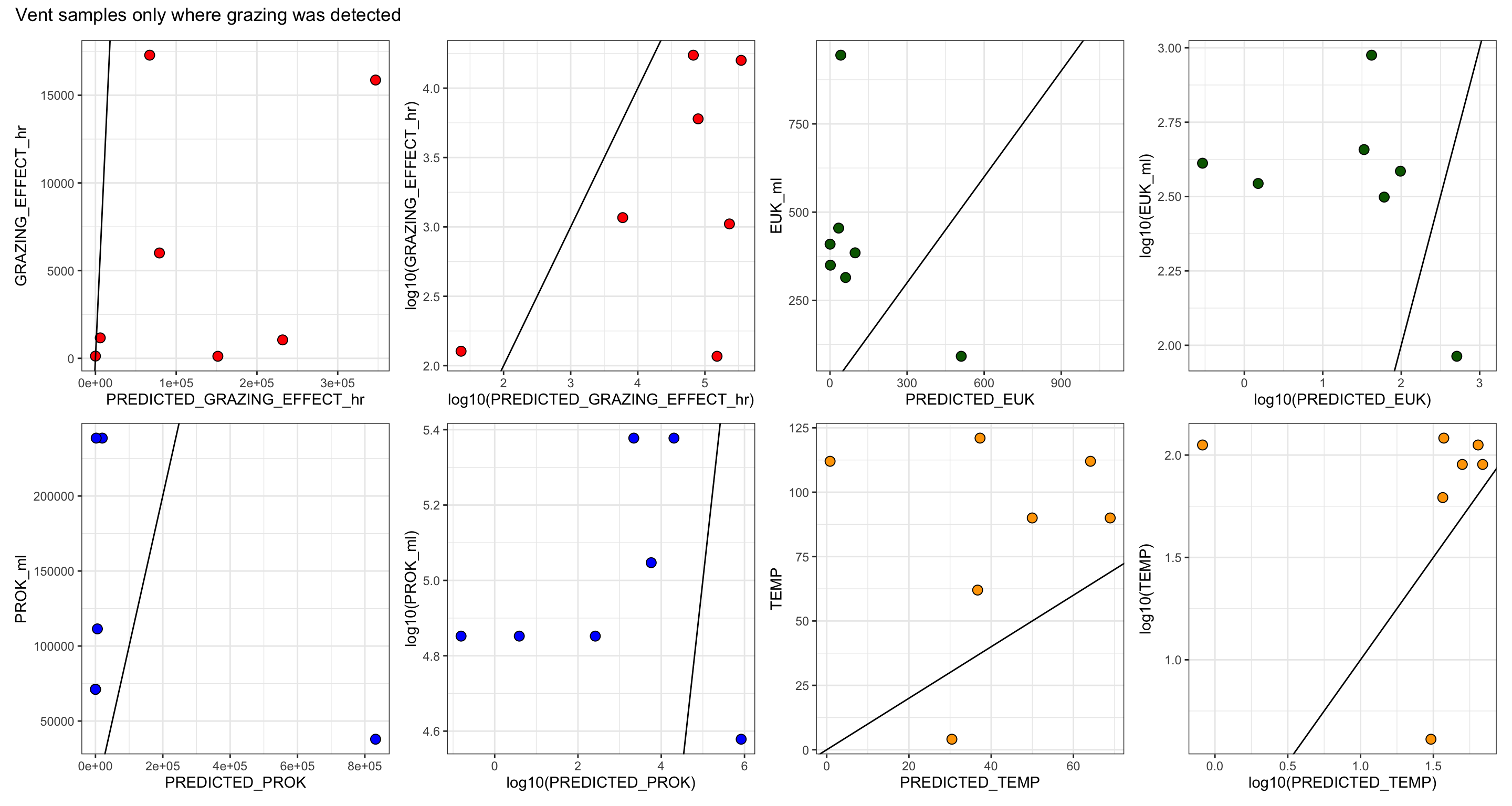

Code

# View(all_vents)
est_predicted(all_vents %>% 
                filter(!(NAME %in% bsw)) %>% 
                filter(FIELD %in% mcr) %>% 
                filter(GRAZING_EFFECT_hr > 0), "MCR vent samples only where grazing was detected")

`summarise()` has grouped output by 'FIELD', 'NAME', 'SAMPLE', 'EXP',
'PROK_ml', 'EUK_ml'. You can override using the `.groups` argument.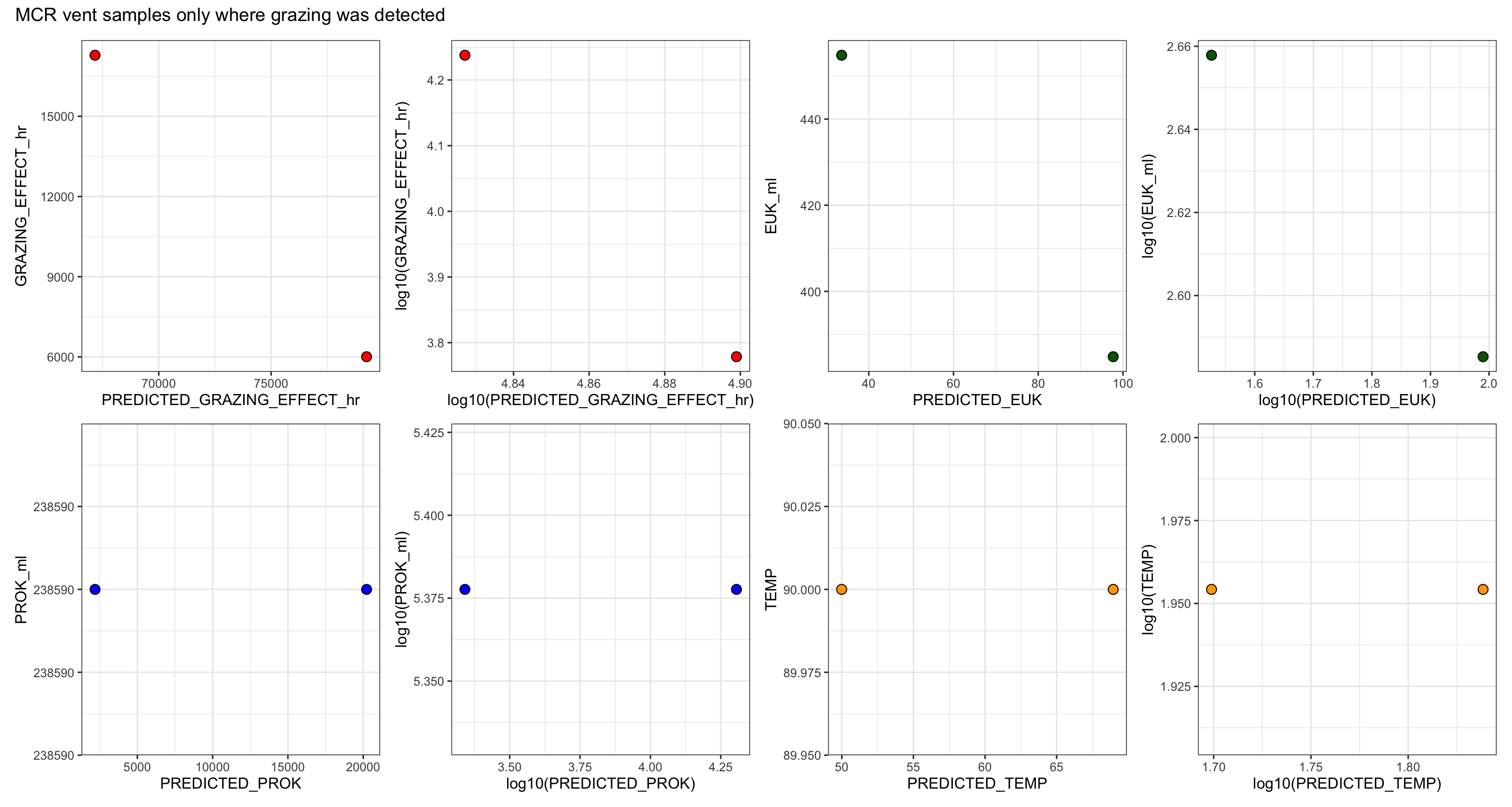

Code

est_predicted(all_vents %>% 
                filter(!(NAME %in% bsw)) %>% 
                filter(FIELD == "Von Damm") %>% 
                filter(GRAZING_EFFECT_hr > 0), "MCR vent samples only where grazing was detected")

`summarise()` has grouped output by 'FIELD', 'NAME', 'SAMPLE', 'EXP',
'PROK_ml', 'EUK_ml'. You can override using the `.groups` argument.

Code

# not really enough in Piccard to make this statistically sound.
# est_predicted(all_vents %>% 
#                 filter(!(NAME %in% bsw)) %>% 
#                 filter(FIELD == "Piccard") %>% 
#                 filter(GRAZING_EFFECT_hr > 0), "MCR vent samples only where grazing was detected")

Code

hist(all_vents$Highest.Temp)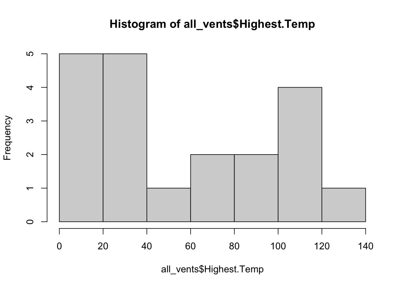

What about a temperature threshold? Perhaps this exists, but maybe not enough data to include.

Code

est_predicted(all_vents %>% 
                # filter(!(NAME %in% bsw)) %>% 
                filter(Highest.Temp > 60), "All samples, temps higher than 60C")

`summarise()` has grouped output by 'FIELD', 'NAME', 'SAMPLE', 'EXP',
'PROK_ml', 'EUK_ml'. You can override using the `.groups` argument.

Warning: Removed 1 rows containing missing values (`geom_point()`).
Removed 1 rows containing missing values (`geom_point()`).
Removed 1 rows containing missing values (`geom_point()`).
Removed 1 rows containing missing values (`geom_point()`).
Removed 1 rows containing missing values (`geom_point()`).
Removed 1 rows containing missing values (`geom_point()`).
Removed 1 rows containing missing values (`geom_point()`).
Removed 1 rows containing missing values (`geom_point()`).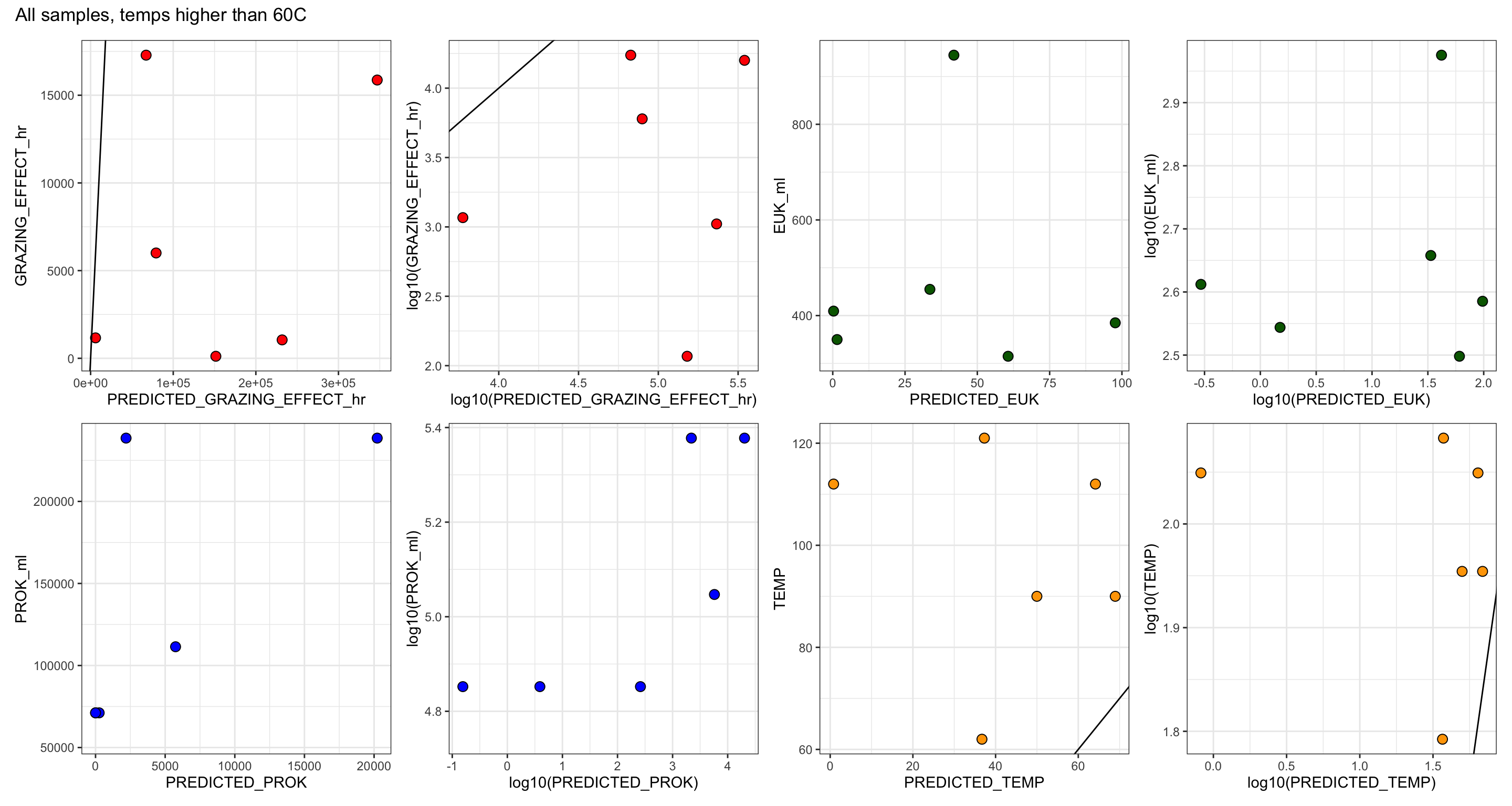

Code

est_predicted(all_vents %>% 
                # filter(!(NAME %in% bsw)) %>% 
                filter(Highest.Temp < 60), "All samples, temps lower than 60C")

`summarise()` has grouped output by 'FIELD', 'NAME', 'SAMPLE', 'EXP',
'PROK_ml', 'EUK_ml'. You can override using the `.groups` argument.

Warning: Removed 3 rows containing missing values (`geom_point()`).

Warning: Removed 3 rows containing missing values (`geom_point()`).
Removed 3 rows containing missing values (`geom_point()`).
Removed 3 rows containing missing values (`geom_point()`).
Removed 3 rows containing missing values (`geom_point()`).
Removed 3 rows containing missing values (`geom_point()`).
Removed 3 rows containing missing values (`geom_point()`).
Removed 3 rows containing missing values (`geom_point()`).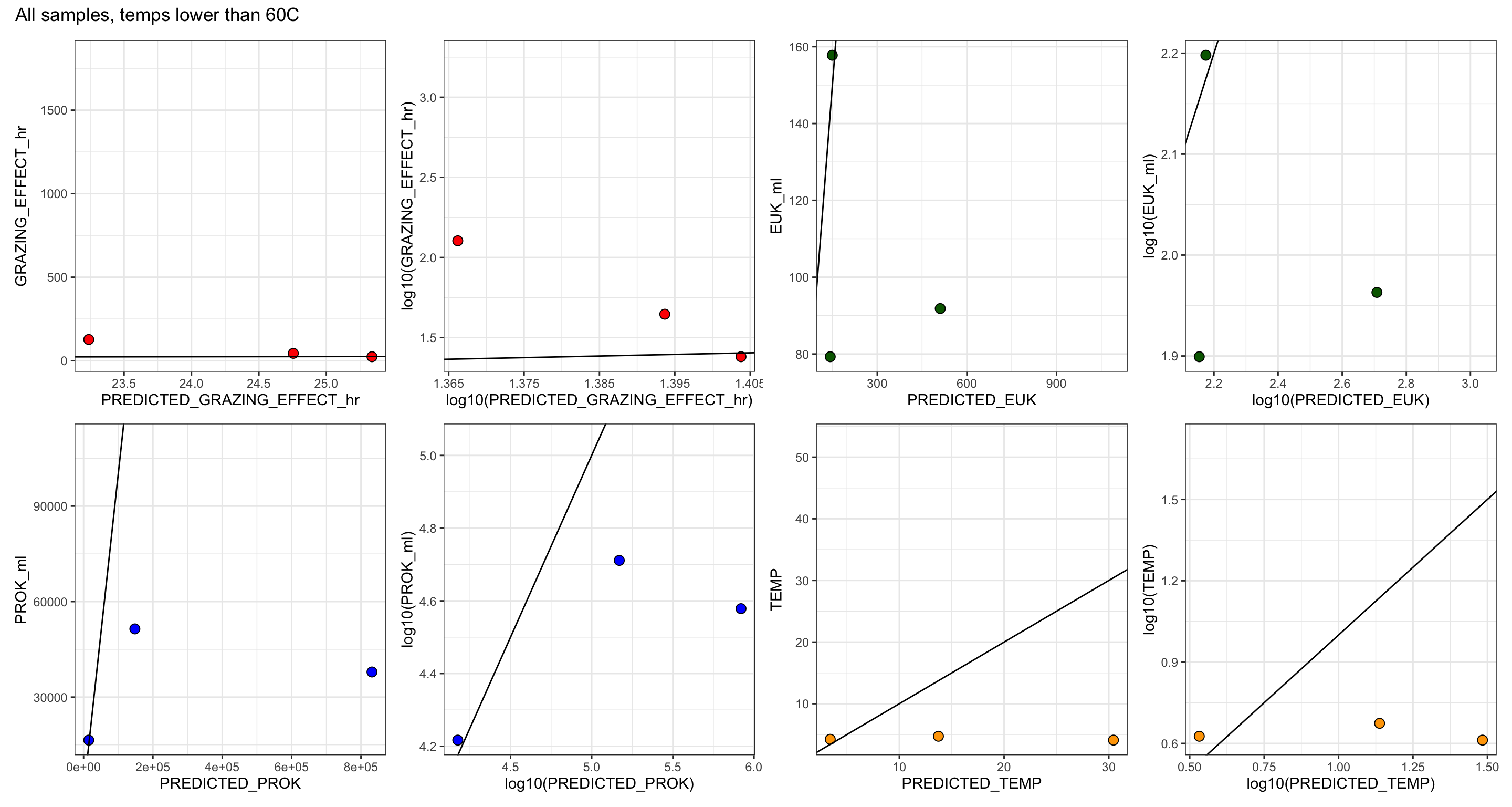

Code

est_predicted(all_vents %>% 
                filter(GRAZING_EFFECT_hr > 0) %>%
                filter(Highest.Temp > 60), "Removed undetected, temps higher than 60C")

`summarise()` has grouped output by 'FIELD', 'NAME', 'SAMPLE', 'EXP',
'PROK_ml', 'EUK_ml'. You can override using the `.groups` argument.

Warning: Removed 1 rows containing missing values (`geom_point()`).
Removed 1 rows containing missing values (`geom_point()`).
Removed 1 rows containing missing values (`geom_point()`).
Removed 1 rows containing missing values (`geom_point()`).
Removed 1 rows containing missing values (`geom_point()`).
Removed 1 rows containing missing values (`geom_point()`).
Removed 1 rows containing missing values (`geom_point()`).
Removed 1 rows containing missing values (`geom_point()`).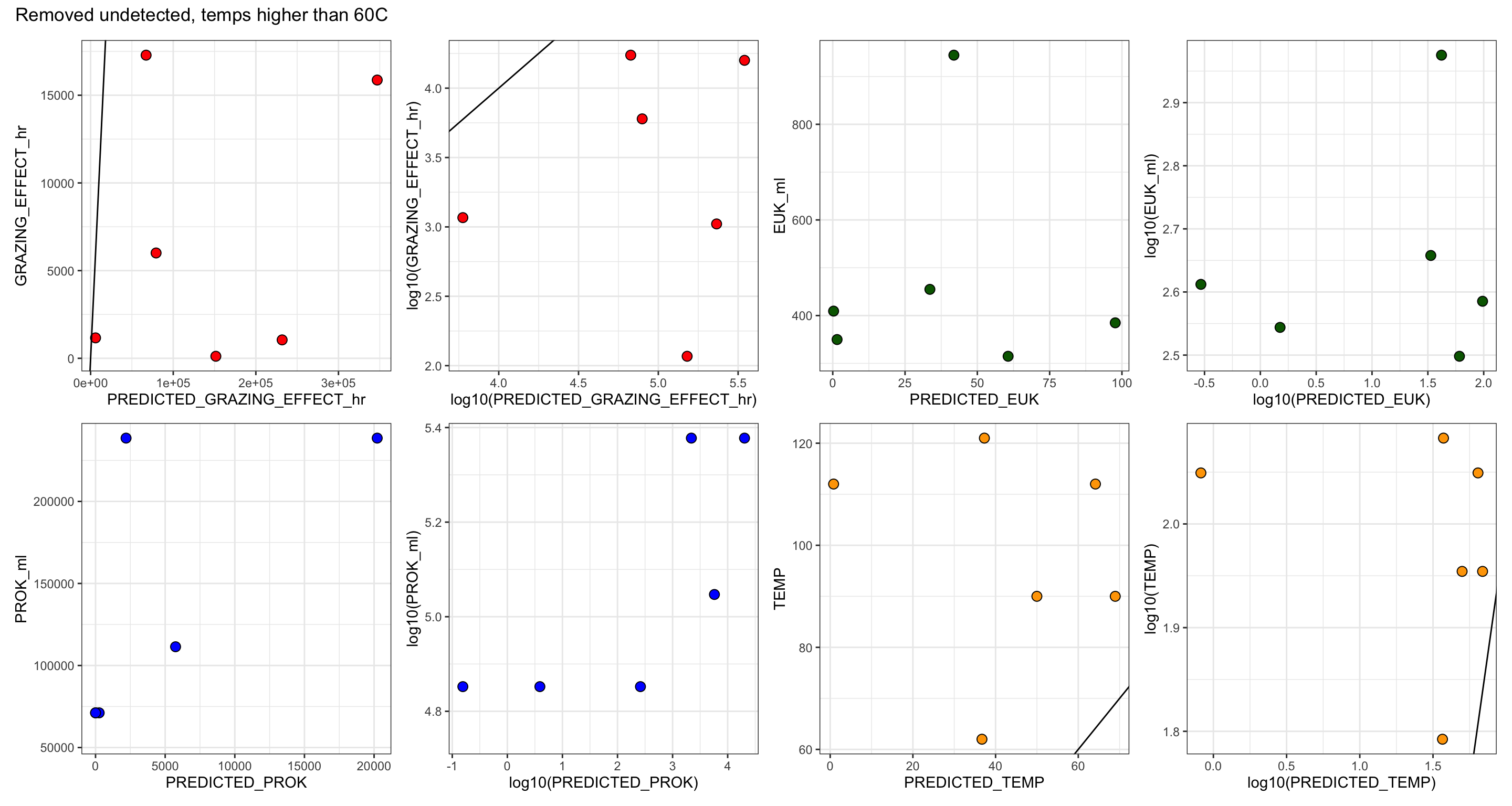

Code

est_predicted(all_vents %>% 
                filter(GRAZING_EFFECT_hr > 0) %>%
                filter(Highest.Temp < 60), "Removed undetected, temps lower than 60C")

`summarise()` has grouped output by 'FIELD', 'NAME', 'SAMPLE', 'EXP',
'PROK_ml', 'EUK_ml'. You can override using the `.groups` argument.

Warning: Removed 3 rows containing missing values (`geom_point()`).

Warning: Removed 3 rows containing missing values (`geom_point()`).
Removed 3 rows containing missing values (`geom_point()`).
Removed 3 rows containing missing values (`geom_point()`).
Removed 3 rows containing missing values (`geom_point()`).
Removed 3 rows containing missing values (`geom_point()`).
Removed 3 rows containing missing values (`geom_point()`).
Removed 3 rows containing missing values (`geom_point()`).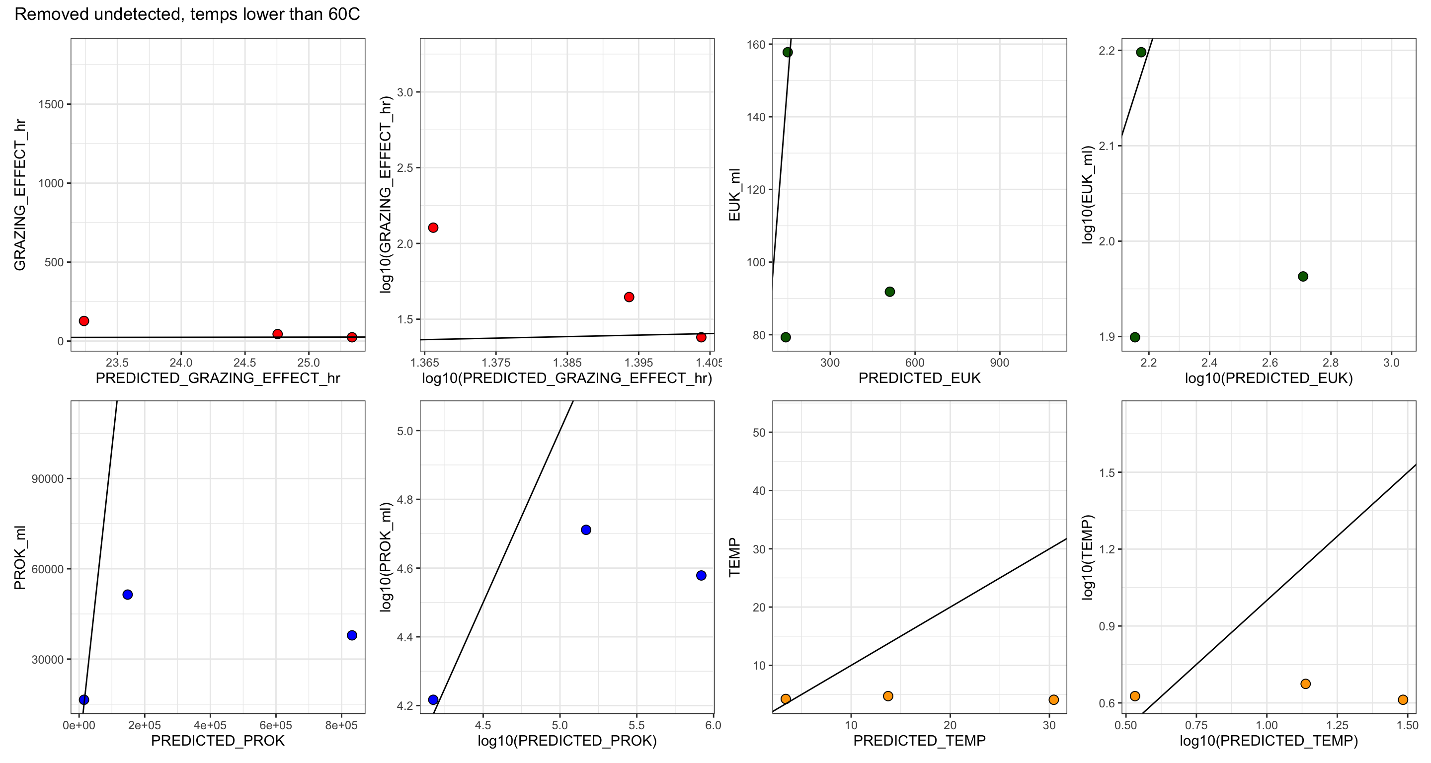

18 Save Robjects for Results

Code

# Oct 22, 2023
save(euk_prok_counts, table_grazerate_wflp_wprok_weuk,
     table_wcalcs, biov_calc, c_factor_biov,
     pgC_ml_biov_bysample, pgC_ml_sizefrac_bysample,
     carbon_consumed, file = "input-data/all-dfs-for-Tables.RData")

19 Session

Code

sessionInfo()

R version 4.3.2 (2023-10-31)
Platform: aarch64-apple-darwin20 (64-bit)
Running under: macOS Sonoma 14.2

Matrix products: default
BLAS:   /Library/Frameworks/R.framework/Versions/4.3-arm64/Resources/lib/libRblas.0.dylib 
LAPACK: /Library/Frameworks/R.framework/Versions/4.3-arm64/Resources/lib/libRlapack.dylib;  LAPACK version 3.11.0

locale:
[1] en_US.UTF-8/en_US.UTF-8/en_US.UTF-8/C/en_US.UTF-8/en_US.UTF-8

time zone: America/Chicago
tzcode source: internal

attached base packages:
[1] stats     graphics  grDevices utils     datasets  methods   base     

other attached packages:
 [1] scales_1.3.0    patchwork_1.2.0 broom_1.0.5     cowplot_1.1.3  
 [5] lubridate_1.9.3 forcats_1.0.0   stringr_1.5.1   dplyr_1.1.4    
 [9] purrr_1.0.2     readr_2.1.5     tidyr_1.3.1     tibble_3.2.1   
[13] ggplot2_3.4.4   tidyverse_2.0.0

loaded via a namespace (and not attached):
 [1] gtable_0.3.4       jsonlite_1.8.8     compiler_4.3.2     tidyselect_1.2.0  
 [5] yaml_2.3.8         fastmap_1.1.1      R6_2.5.1           labeling_0.4.3    
 [9] generics_0.1.3     knitr_1.45         backports_1.4.1    htmlwidgets_1.6.4 
[13] munsell_0.5.0      RColorBrewer_1.1-3 pillar_1.9.0       tzdb_0.4.0        
[17] rlang_1.1.3        utf8_1.2.4         stringi_1.8.3      xfun_0.41         
[21] timechange_0.3.0   cli_3.6.2          withr_3.0.0        magrittr_2.0.3    
[25] digest_0.6.34      grid_4.3.2         rstudioapi_0.15.0  hms_1.1.3         
[29] lifecycle_1.0.4    vctrs_0.6.5        evaluate_0.23      glue_1.7.0        
[33] farver_2.1.1       fansi_1.0.6        colorspace_2.1-0   rmarkdown_2.25    
[37] tools_4.3.2        pkgconfig_2.0.3    htmltools_0.5.7